3.6 Semidefinite Optimization Formulations
53
Constraints (3.90) define the distance between each pair of departments in the
same row. Because the distance between departments i and j is the sum of the
lengths of all the departments between them, there will be no empty space between
adjacent departments, including the dummy departments.
3.6 Semidefinite Optimization Formulations
Semidefinite optimization models have been proposed for the DRFLP and for
several of the variants of the MRFLP presented in this chapter. These models apply
the principles of Sect. 2.7 to derive an SDO approach, but the technical details are
much more involved. Moreover, in most cases, specific solution algorithms must
be implemented to achieve satisfactory performance with the SDO approach. For
this reason, we merely briefly sketch the SDO approach for the k-PROP, and how it
can be applied to instances of the DRFLP and MRFLP. The references provided in
Sect. 3.7 provide all the details.
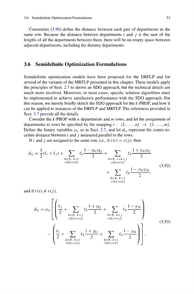
Consider the k-PROP with n departments and m rows, and let the assignment of
departments to rows be specified by the mapping r : {1, . . . , n} → {1, . . . , m}.
Define the binary variables γ ij as in Sect. 2.7, and let d ij represent the centre-tocentre distance between i and j measured parallel to the rows.
If i and j are assigned to the same row, i.e., if r(i) = r(j ), then
d ij =
1
2
(( i + j ) +
k∈N, k r(k)=r(i)
k
1 − γ ki γ kj
2
+
k∈N, i r(k)=r(i)
k
1 + γ ik γ kj
2
+
k∈N, k>j
r(k)=r(i)
k
1 − γ ik γ jk
2
,
(3.92)
and if r(i) = r(j ),
d ij = γ ij
⎡
⎢
⎢
⎣
⎛
⎜
⎜
⎝
j
2
+
k∈N, k r(k)=r(j)
k
1 + γ kj
2
+
k∈N, k>j
r(k)=r(j)
k
1 − γ jk
2
⎞
⎟
⎟
⎠
−
⎛
⎜
⎜
⎝
i
2
+
k∈N, k r(k)=r(i)
k
1 + γ ki
2
+
k∈N, k>i
r(k)=r(i)
k
1 − γ ik
2
⎞
⎟
⎟
⎠
⎤
⎥
⎥
⎦ .
(3.93)