

2.6 Linearizing the Binary Quadratic Optimization Formulation
19
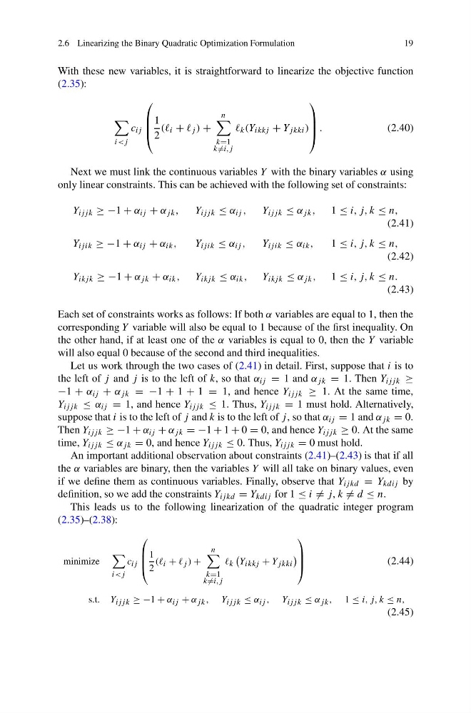
With these new variables, it is straightforward to linearize the objective function
(2.35):
i
⎛
⎜
⎜
⎝
1
2
(( i + j ) +
n
k=1
k =i,j
k (Y ikkj + Y j kki )
⎞
⎟
⎟
⎠ .
(2.40)
Next we must link the continuous variables Y with the binary variables α using
only linear constraints. This can be achieved with the following set of constraints:
Y ijj k ≥ −1 + α ij + α jk , Y ijj k ≤ α ij , Y ijj k ≤ α jk , 1 ≤ i, j, k ≤ n,
(2.41)
Y ij ik ≥ −1 + α ij + α ik ,
Y ij ik ≤ α ij ,
Y ij ik ≤ α ik ,
1 ≤ i, j, k ≤ n,
(2.42)
Y ikj k ≥ −1 + α jk + α ik , Y ikj k ≤ α ik , Y ikj k ≤ α jk , 1 ≤ i, j, k ≤ n.
(2.43)
Each set of constraints works as follows: If both α variables are equal to 1, then the
corresponding Y variable will also be equal to 1 because of the first inequality. On
the other hand, if at least one of the α variables is equal to 0, then the Y variable
will also equal 0 because of the second and third inequalities.
Let us work through the two cases of (2.41) in detail. First, suppose that i is to
the left of j and j is to the left of k, so that α ij = 1 and α jk = 1. Then Y ijj k ≥
−1 + α ij + α jk = −1 + 1 + 1 = 1, and hence Y ijj k ≥ 1. At the same time,
Y ijj k ≤ α ij = 1, and hence Y ijj k ≤ 1. Thus, Y ijj k = 1 must hold. Alternatively,
suppose that i is to the left of j and k is to the left of j , so that α ij = 1 and α jk = 0.
Then Y ijj k ≥ −1 + α ij + α jk = −1 + 1 + 0 = 0, and hence Y ijj k ≥ 0. At the same
time, Y ijj k ≤ α jk = 0, and hence Y ijj k ≤ 0. Thus, Y ijj k = 0 must hold.
An important additional observation about constraints (2.41)–(2.43) is that if all
the α variables are binary, then the variables Y will all take on binary values, even
if we define them as continuous variables. Finally, observe that Y ij kd = Y kdij by
definition, so we add the constraints Y ij kd = Y kdij for 1 ≤ i = j, k = d ≤ n.
This leads us to the following linearization of the quadratic integer program
(2.35)–(2.38):
minimize
i
⎛
⎜
⎜
⎝
1
2
(( i + j ) +
n
k=1
k =i,j
k
Y ikkj + Y j kki
⎞
⎟
⎟
⎠
(2.44)
s.t. Y ijj k ≥ −1 + α ij + α jk , Y ijj k ≤ α ij , Y ijj k ≤ α jk , 1 ≤ i, j, k ≤ n,
(2.45)
19
With these new variables, it is straightforward to linearize the objective function
(2.35):
i
⎛
⎜
⎜
⎝
1
2
(( i + j ) +
n
k=1
k =i,j
k (Y ikkj + Y j kki )
⎞
⎟
⎟
⎠ .
(2.40)
Next we must link the continuous variables Y with the binary variables α using
only linear constraints. This can be achieved with the following set of constraints:
Y ijj k ≥ −1 + α ij + α jk , Y ijj k ≤ α ij , Y ijj k ≤ α jk , 1 ≤ i, j, k ≤ n,
(2.41)
Y ij ik ≥ −1 + α ij + α ik ,
Y ij ik ≤ α ij ,
Y ij ik ≤ α ik ,
1 ≤ i, j, k ≤ n,
(2.42)
Y ikj k ≥ −1 + α jk + α ik , Y ikj k ≤ α ik , Y ikj k ≤ α jk , 1 ≤ i, j, k ≤ n.
(2.43)
Each set of constraints works as follows: If both α variables are equal to 1, then the
corresponding Y variable will also be equal to 1 because of the first inequality. On
the other hand, if at least one of the α variables is equal to 0, then the Y variable
will also equal 0 because of the second and third inequalities.
Let us work through the two cases of (2.41) in detail. First, suppose that i is to
the left of j and j is to the left of k, so that α ij = 1 and α jk = 1. Then Y ijj k ≥
−1 + α ij + α jk = −1 + 1 + 1 = 1, and hence Y ijj k ≥ 1. At the same time,
Y ijj k ≤ α ij = 1, and hence Y ijj k ≤ 1. Thus, Y ijj k = 1 must hold. Alternatively,
suppose that i is to the left of j and k is to the left of j , so that α ij = 1 and α jk = 0.
Then Y ijj k ≥ −1 + α ij + α jk = −1 + 1 + 0 = 0, and hence Y ijj k ≥ 0. At the same
time, Y ijj k ≤ α jk = 0, and hence Y ijj k ≤ 0. Thus, Y ijj k = 0 must hold.
An important additional observation about constraints (2.41)–(2.43) is that if all
the α variables are binary, then the variables Y will all take on binary values, even
if we define them as continuous variables. Finally, observe that Y ij kd = Y kdij by
definition, so we add the constraints Y ij kd = Y kdij for 1 ≤ i = j, k = d ≤ n.
This leads us to the following linearization of the quadratic integer program
(2.35)–(2.38):
minimize
i
⎛
⎜
⎜
⎝
1
2
(( i + j ) +
n
k=1
k =i,j
k
Y ikkj + Y j kki
⎞
⎟
⎟
⎠
(2.44)
s.t. Y ijj k ≥ −1 + α ij + α jk , Y ijj k ≤ α ij , Y ijj k ≤ α jk , 1 ≤ i, j, k ≤ n,
(2.45)