

3.1 Structured Bodies
85
The different versions of the quantum Monte Carlo method all share the common
use of the technique to build accurate estimates to the multidimensional integrals
that arise in the different formulations of the many-body problem. The quantum
Monte Carlo methods allow for a direct treatment and description of complex manybody effects encoded in the wavefunction and offer numerically accurate solutions
of the many-body problem. In principle, any physical system can be described by
the many-body Schrödinger equation provided that the constituent particles are not
moving at a speed comparable to that of light and that, therefore, relativistic effects
can be neglected.
There are, indeed, two versions of the Monte Carlo technique that have been
applied to electronic structure problems: the variational (VMC) and the diffusion
(DMC) one.
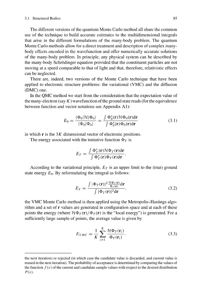
In the QMC method we start from the consideration that the expectation value of
the many-electron (say K ) wavefunction of the ground state reads (for the equivalence
between function and vector notations see Appendix A1):
E 0 =
0 |H| 0
0 | 0
=
∗
0 (r)H 0 (r)dr
∗
0 (r)) 0 (r)dr
(3.1)
in which r is the 3K dimensional vector of electronic positions.
The energy associated with the tentative function T is
E T =
∗
T (r)H T (r)dr
∗
T (r)) T (r)dr
.
According to the variational principle, E T is an upper limit to the (true) ground
state energy E 0 . By reformulating the integral as follows:
E T =
| T (r)|
2 H T (r)
T (r)
dr
| T (r)| 2 dr
.
(3.2)
the VMC Monte Carlo method is then applied using the Metropolis–Hastings algorithm and a set of r values are generated in configuration space and at each of these
points the energy (where H T (r)// T (r) is the “local energy”) is generated. For a
sufficiently large sample of points, the average value is given by
E V MC =
1
K
K
i=1
H T (r i )
T (r i )
.
(3.3)
the next iteration) or rejected (in which case the candidate value is discarded, and current value is
reused in the next iteration). The probability of acceptance is determined by comparing the values of
the function f (x) of the current and candidate sample values with respect to the desired distribution
P(x).
85
The different versions of the quantum Monte Carlo method all share the common
use of the technique to build accurate estimates to the multidimensional integrals
that arise in the different formulations of the many-body problem. The quantum
Monte Carlo methods allow for a direct treatment and description of complex manybody effects encoded in the wavefunction and offer numerically accurate solutions
of the many-body problem. In principle, any physical system can be described by
the many-body Schrödinger equation provided that the constituent particles are not
moving at a speed comparable to that of light and that, therefore, relativistic effects
can be neglected.
There are, indeed, two versions of the Monte Carlo technique that have been
applied to electronic structure problems: the variational (VMC) and the diffusion
(DMC) one.
In the QMC method we start from the consideration that the expectation value of
the many-electron (say K ) wavefunction of the ground state reads (for the equivalence
between function and vector notations see Appendix A1):
E 0 =
0 |H| 0
0 | 0
=
∗
0 (r)H 0 (r)dr
∗
0 (r)) 0 (r)dr
(3.1)
in which r is the 3K dimensional vector of electronic positions.
The energy associated with the tentative function T is
E T =
∗
T (r)H T (r)dr
∗
T (r)) T (r)dr
.
According to the variational principle, E T is an upper limit to the (true) ground
state energy E 0 . By reformulating the integral as follows:
E T =
| T (r)|
2 H T (r)
T (r)
dr
| T (r)| 2 dr
.
(3.2)
the VMC Monte Carlo method is then applied using the Metropolis–Hastings algorithm and a set of r values are generated in configuration space and at each of these
points the energy (where H T (r)// T (r) is the “local energy”) is generated. For a
sufficiently large sample of points, the average value is given by
E V MC =
1
K
K
i=1
H T (r i )
T (r i )
.
(3.3)
the next iteration) or rejected (in which case the candidate value is discarded, and current value is
reused in the next iteration). The probability of acceptance is determined by comparing the values of
the function f (x) of the current and candidate sample values with respect to the desired distribution
P(x).