

2.1 Quantum Mechanics and Bound States
47
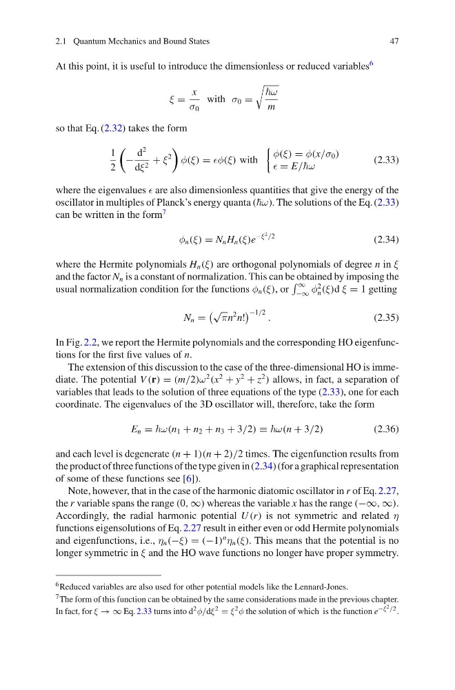
At this point, it is useful to introduce the dimensionless or reduced variables
6
ξ =
x
σ 0
with σ 0 =
ω
m
so that Eq. (2.32) takes the form
1
2
−
d
2
dξ 2 + ξ
2
φ(ξ) = φ(ξ) with
φ(ξ) = φ(x/σ 0 )
= E/ω
(2.33)
where the eigenvalues are also dimensionless quantities that give the energy of the
oscillator in multiples of Planck’s energy quanta (ω). The solutions of the Eq. (2.33)
can be written in the form
7
φ n (ξ) = N n H n (ξ)e
−ξ
2 /2
(2.34)
where the Hermite polynomials H n (ξ) are orthogonal polynomials of degree n in ξ
and the factor N n is a constant of normalization. This can be obtained by imposing the
usual normalization condition for the functions φ n (ξ), or
∞
−∞ φ
2
n (ξ)d ξ = 1 getting
N n =
√
πn
2 n!
−1/2 .
(2.35)
In Fig. 2.2, we report the Hermite polynomials and the corresponding HO eigenfunctions for the first five values of n.
The extension of this discussion to the case of the three-dimensional HO is immediate. The potential V (r) = (m/2)ω
2
(x
2
+ y
2
+ z
2
) allows, in fact, a separation of
variables that leads to the solution of three equations of the type (2.33), one for each
coordinate. The eigenvalues of the 3D oscillator will, therefore, take the form
E n = ω(n 1 + n 2 + n 3 + 3/2) ≡ ω(n + 3/2)
(2.36)
and each level is degenerate (n + 1)(n + 2)/2 times. The eigenfunction results from
the product of three functions of the type given in (2.34) (for a graphical representation
of some of these functions see [6]).
Note, however, that in the case of the harmonic diatomic oscillator in r of Eq. 2.27,
the r variable spans the range (0, ∞) whereas the variable x has the range (−∞, ∞).
Accordingly, the radial harmonic potential U (r) is not symmetric and related η
functions eigensolutions of Eq. 2.27 result in either even or odd Hermite polynomials
and eigenfunctions, i.e., η n (−ξ) = (−1)
n
η n (ξ). This means that the potential is no
longer symmetric in ξ and the HO wave functions no longer have proper symmetry.
6 Reduced variables are also used for other potential models like the Lennard-Jones.
7 The form of this function can be obtained by the same considerations made in the previous chapter.
In fact, for ξ → ∞ Eq. 2.33 turns into d 2 φ/dξ 2 = ξ 2 φ the solution of which is the function e −ξ 2 /2 .
47
At this point, it is useful to introduce the dimensionless or reduced variables
6
ξ =
x
σ 0
with σ 0 =
ω
m
so that Eq. (2.32) takes the form
1
2
−
d
2
dξ 2 + ξ
2
φ(ξ) = φ(ξ) with
φ(ξ) = φ(x/σ 0 )
= E/ω
(2.33)
where the eigenvalues are also dimensionless quantities that give the energy of the
oscillator in multiples of Planck’s energy quanta (ω). The solutions of the Eq. (2.33)
can be written in the form
7
φ n (ξ) = N n H n (ξ)e
−ξ
2 /2
(2.34)
where the Hermite polynomials H n (ξ) are orthogonal polynomials of degree n in ξ
and the factor N n is a constant of normalization. This can be obtained by imposing the
usual normalization condition for the functions φ n (ξ), or
∞
−∞ φ
2
n (ξ)d ξ = 1 getting
N n =
√
πn
2 n!
−1/2 .
(2.35)
In Fig. 2.2, we report the Hermite polynomials and the corresponding HO eigenfunctions for the first five values of n.
The extension of this discussion to the case of the three-dimensional HO is immediate. The potential V (r) = (m/2)ω
2
(x
2
+ y
2
+ z
2
) allows, in fact, a separation of
variables that leads to the solution of three equations of the type (2.33), one for each
coordinate. The eigenvalues of the 3D oscillator will, therefore, take the form
E n = ω(n 1 + n 2 + n 3 + 3/2) ≡ ω(n + 3/2)
(2.36)
and each level is degenerate (n + 1)(n + 2)/2 times. The eigenfunction results from
the product of three functions of the type given in (2.34) (for a graphical representation
of some of these functions see [6]).
Note, however, that in the case of the harmonic diatomic oscillator in r of Eq. 2.27,
the r variable spans the range (0, ∞) whereas the variable x has the range (−∞, ∞).
Accordingly, the radial harmonic potential U (r) is not symmetric and related η
functions eigensolutions of Eq. 2.27 result in either even or odd Hermite polynomials
and eigenfunctions, i.e., η n (−ξ) = (−1)
n
η n (ξ). This means that the potential is no
longer symmetric in ξ and the HO wave functions no longer have proper symmetry.
6 Reduced variables are also used for other potential models like the Lennard-Jones.
7 The form of this function can be obtained by the same considerations made in the previous chapter.
In fact, for ξ → ∞ Eq. 2.33 turns into d 2 φ/dξ 2 = ξ 2 φ the solution of which is the function e −ξ 2 /2 .