

4.3 Beyond Full Quantum Calculations
135
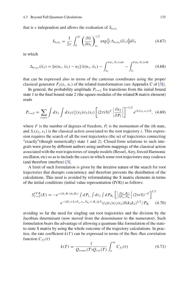
that is v independent and allows the evaluation of S n 1 n 2
S n 1 n 2 =
1
2π
2π
0
∂α
∂α 1
1/2
n 1
exp
i n 1 n 2 (α 1 )
dα 1
(4.67)
in which
n 1 n 2 (α 1 ) = [n(n 1 , α 1 ) − n 2 ] α(n 1 , α 1 ) −
n(n 1 ,α 1 )αdn
n 1
−
k(n 1 ,α 1 )rdk
k 1
(4.68)
that can be expressed also in terms of the cartesian coordinates using the proper
classical generator F 2 (x i , n i ) of the related transformation (see Appendix C of [3]).
In general, the probability amplitude P 1→2 for transitions from the initial bound
state 1 to the final bound state 2 (the square modulus of the related S matrix element)
reads
P 1→2 =
roots
dx 1
dx 2 ψ
∗
2 (x 2 )ψ 1 (x 1 )
(2πi)
F
∂x 2
∂ P 1
−1/2
e
i S i (x 2 ,x 1 )/
, (4.69)
where F is the number of degrees of freedom, P i is the momentum of the ith state,
and S i (x 2 , x 1 ) is the classical action associated to the root trajectory i. This expression requires the search of all the root trajectories (the set of trajectories connecting
“exactly”(though numerically) state 1 and 2). Closed-form solutions to such integrals were given by different authors using uniform mappings of the classical action
associated with the root trajectories of simple models (Bessel, Airy, forced Harmonic
oscillator, etc) so as to include the cases in which some root trajectories may coalesce
(and therefore interfere) [3].
A limit of such formulation is given by the iterative nature of the search for root
trajectories that disrupts concurrency and therefore prevents the distribution of the
calculations. This need is avoided by reformulating the S matrix elements in terms
of the initial conditions (initial value representation (IVR)) as follows:
S
I V R
1→2 (E) = −e
−i(k 1 R 1 +k 2 R 2 )
d P r o
dr o
d P R o
∂(r t ,R t )
∂ P ro ,P Ro
(2πi)
−F
1/2
e
−i[E t +S t (P ro ,r o ,P Ro +,R o )]/
ψ 2 (r t )ψ 1 (r o )(k 2 k 1 )
1/2
/P R t
(4.70)
avoiding so far the need for singling out root trajectories and the division by the
Jacobian determinant (now moved from the denominator to the numerator). Such
formulation bears the advantage of allowing a quantum-like formulation of the stateto-state S matrix by using the whole outcome of the trajectory calculations. In practice, the rate coefficient k(T ) can be expressed in terms of the flux–flux correlation
function C f f (t)
k(T ) =
1
Q trans (T )Q rot (T )
∞
o
C f f (t)
(4.71)
135
that is v independent and allows the evaluation of S n 1 n 2
S n 1 n 2 =
1
2π
2π
0
∂α
∂α 1
1/2
n 1
exp
i n 1 n 2 (α 1 )
dα 1
(4.67)
in which
n 1 n 2 (α 1 ) = [n(n 1 , α 1 ) − n 2 ] α(n 1 , α 1 ) −
n(n 1 ,α 1 )αdn
n 1
−
k(n 1 ,α 1 )rdk
k 1
(4.68)
that can be expressed also in terms of the cartesian coordinates using the proper
classical generator F 2 (x i , n i ) of the related transformation (see Appendix C of [3]).
In general, the probability amplitude P 1→2 for transitions from the initial bound
state 1 to the final bound state 2 (the square modulus of the related S matrix element)
reads
P 1→2 =
roots
dx 1
dx 2 ψ
∗
2 (x 2 )ψ 1 (x 1 )
(2πi)
F
∂x 2
∂ P 1
−1/2
e
i S i (x 2 ,x 1 )/
, (4.69)
where F is the number of degrees of freedom, P i is the momentum of the ith state,
and S i (x 2 , x 1 ) is the classical action associated to the root trajectory i. This expression requires the search of all the root trajectories (the set of trajectories connecting
“exactly”(though numerically) state 1 and 2). Closed-form solutions to such integrals were given by different authors using uniform mappings of the classical action
associated with the root trajectories of simple models (Bessel, Airy, forced Harmonic
oscillator, etc) so as to include the cases in which some root trajectories may coalesce
(and therefore interfere) [3].
A limit of such formulation is given by the iterative nature of the search for root
trajectories that disrupts concurrency and therefore prevents the distribution of the
calculations. This need is avoided by reformulating the S matrix elements in terms
of the initial conditions (initial value representation (IVR)) as follows:
S
I V R
1→2 (E) = −e
−i(k 1 R 1 +k 2 R 2 )
d P r o
dr o
d P R o
∂(r t ,R t )
∂ P ro ,P Ro
(2πi)
−F
1/2
e
−i[E t +S t (P ro ,r o ,P Ro +,R o )]/
ψ 2 (r t )ψ 1 (r o )(k 2 k 1 )
1/2
/P R t
(4.70)
avoiding so far the need for singling out root trajectories and the division by the
Jacobian determinant (now moved from the denominator to the numerator). Such
formulation bears the advantage of allowing a quantum-like formulation of the stateto-state S matrix by using the whole outcome of the trajectory calculations. In practice, the rate coefficient k(T ) can be expressed in terms of the flux–flux correlation
function C f f (t)
k(T ) =
1
Q trans (T )Q rot (T )
∞
o
C f f (t)
(4.71)