

72
3 Two (or More) Magnetic Centers
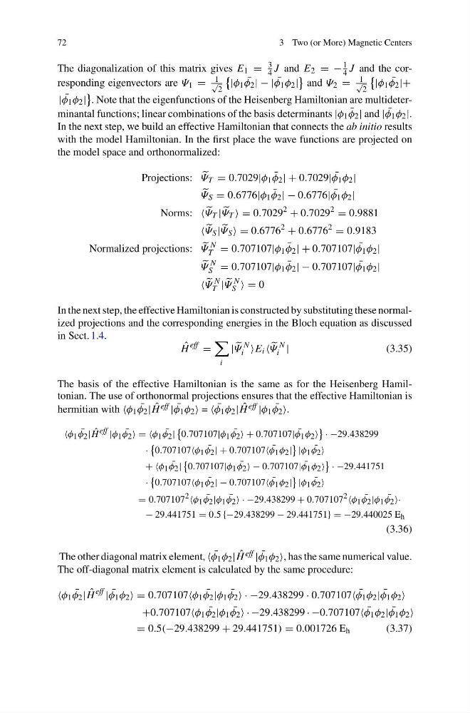
The diagonalization of this matrix gives E 1 =
3
4 J and E 2 =−
1
4 J and the corresponding eigenvectors are Ψ 1 =
1
√
2
|φ 1 ¯
φ 2 |−| ¯
φ 1 φ 2 |
and Ψ 2 =
1
√
2
|φ 1 ¯
φ 2 |+
| ¯
φ 1 φ 2 |
. Note that the eigenfunctions of the Heisenberg Hamiltonian are multideterminantal functions; linear combinations of the basis determinants |φ 1 ¯
φ 2 | and | ¯
φ 1 φ 2 |.
In the next step, we build an effective Hamiltonian that connects the ab initio results
with the model Hamiltonian. In the first place the wave functions are projected on
the model space and orthonormalized:
Projections:
Ψ T = 0.7029|φ 1 ¯
φ 2 |+0.7029| ¯
φ 1 φ 2 |
Ψ S = 0.6776|φ 1 ¯
φ 2 |−0.6776| ¯
φ 1 φ 2 |
Norms:
Ψ T |
Ψ T =0.7029
2 + 0.7029
2 = 0.9881
Ψ S |
Ψ S =0.6776
2 + 0.6776
2 = 0.9183
Normalized projections:
Ψ
N
T = 0.707107|φ 1 ¯
φ 2 |+0.707107| ¯
φ 1 φ 2 |
Ψ
N
S = 0.707107|φ 1 ¯
φ 2 |−0.707107| ¯
φ 1 φ 2 |
Ψ
N
T |
Ψ
N
S =0
In the next step, the effective Hamiltonian is constructed by substituting these normalized projections and the corresponding energies in the Bloch equation as discussed
in Sect. 1.4.
ˆ
H
eff =
i
|
Ψ
N
i E i
Ψ
N
i |
(3.35)
The basis of the effective Hamiltonian is the same as for the Heisenberg Hamiltonian. The use of orthonormal projections ensures that the effective Hamiltonian is
hermitian with φ 1 ¯
φ 2 | ˆ
H eff | ¯
φ 1 φ 2 = ¯
φ 1 φ 2 | ˆ
H eff |φ 1 ¯
φ 2 .
φ 1 ¯
φ 2 | ˆ
H eff |φ 1 ¯
φ 2 ==φ 1 ¯
φ 2 |
0.707107|φ 1 ¯
φ 2 +0.707107| ¯
φ 1 φ 2
·−29.438299
·
0.707107φ 1 ¯
φ 2 |+0.707107 ¯
φ 1 φ 2 |
|φ 1 ¯
φ 2
++φ 1 ¯
φ 2 |
0.707107|φ 1 ¯
φ 2 −0.707107| ¯
φ 1 φ 2
·−29.441751
·
0.707107φ 1 ¯
φ 2 |−0.707107 ¯
φ 1 φ 2 |
|φ 1 ¯
φ 2
= 0.707107 2 φ 1 ¯
φ 2 |φ 1 ¯
φ 2 ·−29.438299 + 0.707107 2 φ 1 ¯
φ 2 |φ 1 ¯
φ 2 ·
− 29.441751 = 0.5 {−29.438299 − 29.441751} =−29.440025 E h
(3.36)
The other diagonal matrix element, ¯
φ 1 φ 2 | ˆ
H eff | ¯
φ 1 φ 2 , has the same numerical value.
The off-diagonal matrix element is calculated by the same procedure:
φ 1 ¯
φ 2 | ˆ
H
eff | ¯
φ 1 φ 2 =0.707107φ 1 ¯
φ 2 |φ 1 ¯
φ 2 ·−29.438299 · 0.707107 ¯
φ 1 φ 2 | ¯
φ 1 φ 2
+0.707107φ 1 ¯
φ 2 |φ 1 ¯
φ 2 ·−29.438299 ·−0.707107 ¯
φ 1 φ 2 | ¯
φ 1 φ 2
= 0.5(−29.438299 + 29.441751) = 0.001726 E h
(3.37)
3 Two (or More) Magnetic Centers
The diagonalization of this matrix gives E 1 =
3
4 J and E 2 =−
1
4 J and the corresponding eigenvectors are Ψ 1 =
1
√
2
|φ 1 ¯
φ 2 |−| ¯
φ 1 φ 2 |
and Ψ 2 =
1
√
2
|φ 1 ¯
φ 2 |+
| ¯
φ 1 φ 2 |
. Note that the eigenfunctions of the Heisenberg Hamiltonian are multideterminantal functions; linear combinations of the basis determinants |φ 1 ¯
φ 2 | and | ¯
φ 1 φ 2 |.
In the next step, we build an effective Hamiltonian that connects the ab initio results
with the model Hamiltonian. In the first place the wave functions are projected on
the model space and orthonormalized:
Projections:
Ψ T = 0.7029|φ 1 ¯
φ 2 |+0.7029| ¯
φ 1 φ 2 |
Ψ S = 0.6776|φ 1 ¯
φ 2 |−0.6776| ¯
φ 1 φ 2 |
Norms:
Ψ T |
Ψ T =0.7029
2 + 0.7029
2 = 0.9881
Ψ S |
Ψ S =0.6776
2 + 0.6776
2 = 0.9183
Normalized projections:
Ψ
N
T = 0.707107|φ 1 ¯
φ 2 |+0.707107| ¯
φ 1 φ 2 |
Ψ
N
S = 0.707107|φ 1 ¯
φ 2 |−0.707107| ¯
φ 1 φ 2 |
Ψ
N
T |
Ψ
N
S =0
In the next step, the effective Hamiltonian is constructed by substituting these normalized projections and the corresponding energies in the Bloch equation as discussed
in Sect. 1.4.
ˆ
H
eff =
i
|
Ψ
N
i E i
Ψ
N
i |
(3.35)
The basis of the effective Hamiltonian is the same as for the Heisenberg Hamiltonian. The use of orthonormal projections ensures that the effective Hamiltonian is
hermitian with φ 1 ¯
φ 2 | ˆ
H eff | ¯
φ 1 φ 2 = ¯
φ 1 φ 2 | ˆ
H eff |φ 1 ¯
φ 2 .
φ 1 ¯
φ 2 | ˆ
H eff |φ 1 ¯
φ 2 ==φ 1 ¯
φ 2 |
0.707107|φ 1 ¯
φ 2 +0.707107| ¯
φ 1 φ 2
·−29.438299
·
0.707107φ 1 ¯
φ 2 |+0.707107 ¯
φ 1 φ 2 |
|φ 1 ¯
φ 2
++φ 1 ¯
φ 2 |
0.707107|φ 1 ¯
φ 2 −0.707107| ¯
φ 1 φ 2
·−29.441751
·
0.707107φ 1 ¯
φ 2 |−0.707107 ¯
φ 1 φ 2 |
|φ 1 ¯
φ 2
= 0.707107 2 φ 1 ¯
φ 2 |φ 1 ¯
φ 2 ·−29.438299 + 0.707107 2 φ 1 ¯
φ 2 |φ 1 ¯
φ 2 ·
− 29.441751 = 0.5 {−29.438299 − 29.441751} =−29.440025 E h
(3.36)
The other diagonal matrix element, ¯
φ 1 φ 2 | ˆ
H eff | ¯
φ 1 φ 2 , has the same numerical value.
The off-diagonal matrix element is calculated by the same procedure:
φ 1 ¯
φ 2 | ˆ
H
eff | ¯
φ 1 φ 2 =0.707107φ 1 ¯
φ 2 |φ 1 ¯
φ 2 ·−29.438299 · 0.707107 ¯
φ 1 φ 2 | ¯
φ 1 φ 2
+0.707107φ 1 ¯
φ 2 |φ 1 ¯
φ 2 ·−29.438299 ·−0.707107 ¯
φ 1 φ 2 | ¯
φ 1 φ 2
= 0.5(−29.438299 + 29.441751) = 0.001726 E h
(3.37)