

64
3 Two (or More) Magnetic Centers
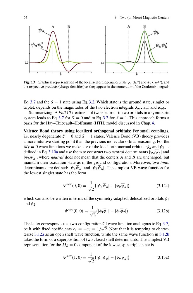
Fig. 3.3 Graphical representation of the localized orthogonal orbitals ψ a (left)andψ b (right), and
the respective products (charge densities) as they appear in the numerator of the Coulomb integrals
Eq. 3.7 and the S = 1 state using Eq. 3.2. Which state is the ground state, singlet or
triplet, depends on the magnitudes of the two electron integrals J aa , J ab and K ab .
Summarizing: A Full CI treatment of two electrons in two orbitals in a symmetric
system leads to Eq. 3.7 for S = 0 and to Eq. 3.2 for S = 1. This approach forms a
basis for the Hay–Thibeault–Hoffmann (HTH) model discussed in Chap. 4.
Valence Bond theory using localized orthogonal orbitals: For small couplings,
i.e. nearly degenerate S = 0 and S = 1 states, Valence Bond (VB) theory provides
a more intuitive starting point than the previous molecular orbital reasoning. For the
M S = 0 wave functions we make use of the local orthonormal orbitals ψ a and ψ b as
defined in Eq. 3.10a and use them to construct two neutral determinants |ψ a ψ b | and
|ψ b ψ a |, where neutral does not mean that the centers A and B are uncharged, but
maintain their oxidation state as in the ground configuration. Moreover, two ionic
determinants are defined: |ψ a ψ a | and |ψ b ψ b |. The simplest VB wave function for
the lowest singlet state has the form
Ψ
cov (0, 0) =
1
√
2
|ψ a ψ b |+|ψ b ψ a |
(3.12a)
which can also be written in terms of the symmetry-adapted, delocalized orbitals φ 1
and φ 2 :
Ψ
cov (0, 0) =
1
√
2
|φ 1 φ 1 |−|φ 2 φ 2 |
(3.12b)
The latter corresponds to a two-configuration CI wave function analogous to Eq. 3.7,
be it with fixed coefficients c 1 =− c 2 = 1/
√
2. Note that it is tempting to characterize 3.12a as an open shell wave function, while the same wave function in 3.12b
takes the form of a superposition of two closed shell determinants. The simplest VB
representation for the M S = 0 component of the lowest spin-triplet state is
Ψ
cov (1, 0) =
1
√
2
|ψ a ψ b |−|ψ b ψ a |
(3.13a)
3 Two (or More) Magnetic Centers
Fig. 3.3 Graphical representation of the localized orthogonal orbitals ψ a (left)andψ b (right), and
the respective products (charge densities) as they appear in the numerator of the Coulomb integrals
Eq. 3.7 and the S = 1 state using Eq. 3.2. Which state is the ground state, singlet or
triplet, depends on the magnitudes of the two electron integrals J aa , J ab and K ab .
Summarizing: A Full CI treatment of two electrons in two orbitals in a symmetric
system leads to Eq. 3.7 for S = 0 and to Eq. 3.2 for S = 1. This approach forms a
basis for the Hay–Thibeault–Hoffmann (HTH) model discussed in Chap. 4.
Valence Bond theory using localized orthogonal orbitals: For small couplings,
i.e. nearly degenerate S = 0 and S = 1 states, Valence Bond (VB) theory provides
a more intuitive starting point than the previous molecular orbital reasoning. For the
M S = 0 wave functions we make use of the local orthonormal orbitals ψ a and ψ b as
defined in Eq. 3.10a and use them to construct two neutral determinants |ψ a ψ b | and
|ψ b ψ a |, where neutral does not mean that the centers A and B are uncharged, but
maintain their oxidation state as in the ground configuration. Moreover, two ionic
determinants are defined: |ψ a ψ a | and |ψ b ψ b |. The simplest VB wave function for
the lowest singlet state has the form
Ψ
cov (0, 0) =
1
√
2
|ψ a ψ b |+|ψ b ψ a |
(3.12a)
which can also be written in terms of the symmetry-adapted, delocalized orbitals φ 1
and φ 2 :
Ψ
cov (0, 0) =
1
√
2
|φ 1 φ 1 |−|φ 2 φ 2 |
(3.12b)
The latter corresponds to a two-configuration CI wave function analogous to Eq. 3.7,
be it with fixed coefficients c 1 =− c 2 = 1/
√
2. Note that it is tempting to characterize 3.12a as an open shell wave function, while the same wave function in 3.12b
takes the form of a superposition of two closed shell determinants. The simplest VB
representation for the M S = 0 component of the lowest spin-triplet state is
Ψ
cov (1, 0) =
1
√
2
|ψ a ψ b |−|ψ b ψ a |
(3.13a)