

52
2 One Magnetic Center
2.10 Demonstrate that the matrix element p − | ˆ
L x |p 0 and all other matrix
elements in Eq. 2.65 are equal to
1
2
√
2. Hint: substitute ˆ
L x by ( ˆ
L + + ˆ
L − )/2
2.3.3 Combining ZFS and the External Magnetic Field
The separate descriptions of the zero-field splitting and the effect of an external
magnetic field on the atomic sublevels can now be combined into a unified description
using the following spin Hamiltonian
ˆ
H = μ B g · H ˆ
S + ˆ
S · D · ˆ
S
(2.66)
In the coordinate frame that diagonalizes g and D, which is assumed to be the same
for both, the spin Hamiltonian simplifies to
ˆ
H = μ B (g x H x ˆ
S x + g y H y ˆ
S y + g z H z S z ) + D
ˆ
S
2
z −
1
3
ˆ
S
2
+ E( ˆ
S
2
x − ˆ
S
2
y ) (2.67)
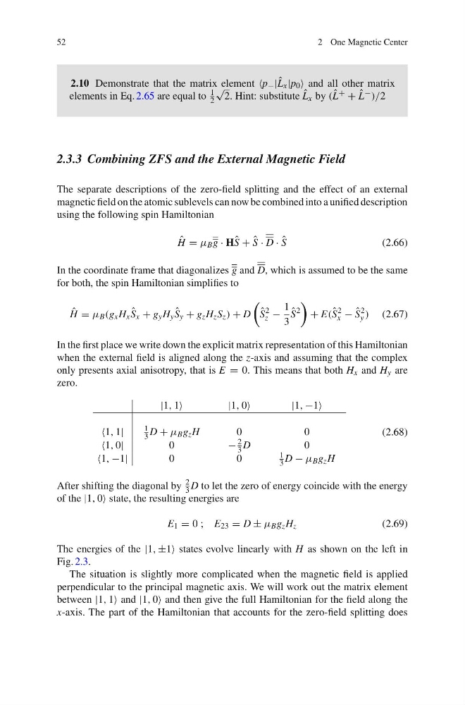
In the first place we write down the explicit matrix representation of this Hamiltonian
when the external field is aligned along the z-axis and assuming that the complex
only presents axial anisotropy, that is E = 0. This means that both H x and H y are
zero.
|1, 1| 1, 0| 1, −1
1, 1|
1
3 D + μ B g z H
00
1, 0|
0
−
2
3 D
0
1, −1|
00
1
3 D − μ B g z H
(2.68)
After shifting the diagonal by
2
3 D to let the zero of energy coincide with the energy
of the |1, 0 state, the resulting energies are
E 1 = 0; E 23 = D ± μ B g z H z
(2.69)
The energies of the |1, ±1 states evolve linearly with H as shown on the left in
Fig. 2.3.
The situation is slightly more complicated when the magnetic field is applied
perpendicular to the principal magnetic axis. We will work out the matrix element
between |1, 1 and |1, 0 and then give the full Hamiltonian for the field along the
x-axis. The part of the Hamiltonian that accounts for the zero-field splitting does
2 One Magnetic Center
2.10 Demonstrate that the matrix element p − | ˆ
L x |p 0 and all other matrix
elements in Eq. 2.65 are equal to
1
2
√
2. Hint: substitute ˆ
L x by ( ˆ
L + + ˆ
L − )/2
2.3.3 Combining ZFS and the External Magnetic Field
The separate descriptions of the zero-field splitting and the effect of an external
magnetic field on the atomic sublevels can now be combined into a unified description
using the following spin Hamiltonian
ˆ
H = μ B g · H ˆ
S + ˆ
S · D · ˆ
S
(2.66)
In the coordinate frame that diagonalizes g and D, which is assumed to be the same
for both, the spin Hamiltonian simplifies to
ˆ
H = μ B (g x H x ˆ
S x + g y H y ˆ
S y + g z H z S z ) + D
ˆ
S
2
z −
1
3
ˆ
S
2
+ E( ˆ
S
2
x − ˆ
S
2
y ) (2.67)
In the first place we write down the explicit matrix representation of this Hamiltonian
when the external field is aligned along the z-axis and assuming that the complex
only presents axial anisotropy, that is E = 0. This means that both H x and H y are
zero.
|1, 1| 1, 0| 1, −1
1, 1|
1
3 D + μ B g z H
00
1, 0|
0
−
2
3 D
0
1, −1|
00
1
3 D − μ B g z H
(2.68)
After shifting the diagonal by
2
3 D to let the zero of energy coincide with the energy
of the |1, 0 state, the resulting energies are
E 1 = 0; E 23 = D ± μ B g z H z
(2.69)
The energies of the |1, ±1 states evolve linearly with H as shown on the left in
Fig. 2.3.
The situation is slightly more complicated when the magnetic field is applied
perpendicular to the principal magnetic axis. We will work out the matrix element
between |1, 1 and |1, 0 and then give the full Hamiltonian for the field along the
x-axis. The part of the Hamiltonian that accounts for the zero-field splitting does