

50
2 One Magnetic Center
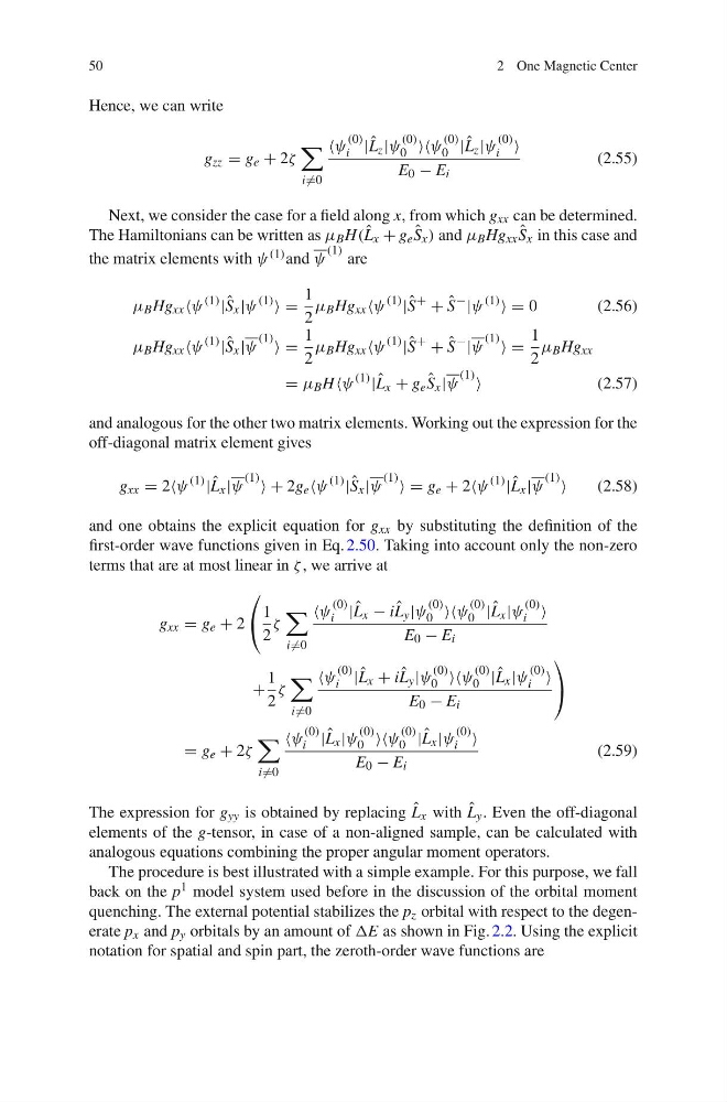
Hence, we can write
g zz = g e + 2ζ
i =0
ψ
(0)
i | ˆ
L z |ψ
(0)
0 ψ
(0)
0 | ˆ
L z |ψ
(0)
i
E 0 − E i
(2.55)
Next, we consider the case for a field along x, from which g xx can be determined.
The Hamiltonians can be written as μ B H( ˆ
L x + g e ˆ
S x ) and μ B Hg xx ˆ
S x in this case and
the matrix elements with ψ (1) and ψ
(1) are
μ B Hg xx ψ
(1) | ˆ
S x |ψ
(1) =
1
2
μ B Hg xx ψ
(1) | ˆ
S
+ + ˆ
S
− |ψ
(1) =0
(2.56)
μ B Hg xx ψ
(1) | ˆ
S x |ψ
(1) =
1
2
μ B Hg xx ψ
(1) | ˆ
S
+ + ˆ
S
− |ψ
(1) =
1
2
μ B Hg xx
= μ B Hψ
(1) | ˆ
L x + g e ˆ
S x |ψ
(1)
(2.57)
and analogous for the other two matrix elements. Working out the expression for the
off-diagonal matrix element gives
g xx = 2ψ
(1) | ˆ
L x |ψ
(1) +2g e ψ
(1) | ˆ
S x |ψ
(1) =g e + 2ψ
(1) | ˆ
L x |ψ
(1)
(2.58)
and one obtains the explicit equation for g xx by substituting the definition of the
first-order wave functions given in Eq. 2.50. Taking into account only the non-zero
terms that are at most linear in ζ ,wearriveat
g xx = g e + 2
⎛
⎝ 1
2
ζ
i =0
ψ
(0)
i | ˆ
L x − i ˆ
L y |ψ
(0)
0 ψ
(0)
0 | ˆ
L x |ψ
(0)
i
E 0 − E i
+
1
2
ζ
i =0
ψ
(0)
i | ˆ
L x + i ˆ
L y |ψ
(0)
0 ψ
(0)
0 | ˆ
L x |ψ
(0)
i
E 0 − E i
⎞
⎠
= g e + 2ζ
i =0
ψ
(0)
i | ˆ
L x |ψ
(0)
0 ψ
(0)
0 | ˆ
L x |ψ
(0)
i
E 0 − E i
(2.59)
The expression for g yy is obtained by replacing ˆ
L x with ˆ
L y . Even the off-diagonal
elements of the g-tensor, in case of a non-aligned sample, can be calculated with
analogous equations combining the proper angular moment operators.
The procedure is best illustrated with a simple example. For this purpose, we fall
back on the p 1 model system used before in the discussion of the orbital moment
quenching. The external potential stabilizes the p z orbital with respect to the degenerate p x and p y orbitals by an amount of E as shown in Fig. 2.2. Using the explicit
notation for spatial and spin part, the zeroth-order wave functions are
2 One Magnetic Center
Hence, we can write
g zz = g e + 2ζ
i =0
ψ
(0)
i | ˆ
L z |ψ
(0)
0 ψ
(0)
0 | ˆ
L z |ψ
(0)
i
E 0 − E i
(2.55)
Next, we consider the case for a field along x, from which g xx can be determined.
The Hamiltonians can be written as μ B H( ˆ
L x + g e ˆ
S x ) and μ B Hg xx ˆ
S x in this case and
the matrix elements with ψ (1) and ψ
(1) are
μ B Hg xx ψ
(1) | ˆ
S x |ψ
(1) =
1
2
μ B Hg xx ψ
(1) | ˆ
S
+ + ˆ
S
− |ψ
(1) =0
(2.56)
μ B Hg xx ψ
(1) | ˆ
S x |ψ
(1) =
1
2
μ B Hg xx ψ
(1) | ˆ
S
+ + ˆ
S
− |ψ
(1) =
1
2
μ B Hg xx
= μ B Hψ
(1) | ˆ
L x + g e ˆ
S x |ψ
(1)
(2.57)
and analogous for the other two matrix elements. Working out the expression for the
off-diagonal matrix element gives
g xx = 2ψ
(1) | ˆ
L x |ψ
(1) +2g e ψ
(1) | ˆ
S x |ψ
(1) =g e + 2ψ
(1) | ˆ
L x |ψ
(1)
(2.58)
and one obtains the explicit equation for g xx by substituting the definition of the
first-order wave functions given in Eq. 2.50. Taking into account only the non-zero
terms that are at most linear in ζ ,wearriveat
g xx = g e + 2
⎛
⎝ 1
2
ζ
i =0
ψ
(0)
i | ˆ
L x − i ˆ
L y |ψ
(0)
0 ψ
(0)
0 | ˆ
L x |ψ
(0)
i
E 0 − E i
+
1
2
ζ
i =0
ψ
(0)
i | ˆ
L x + i ˆ
L y |ψ
(0)
0 ψ
(0)
0 | ˆ
L x |ψ
(0)
i
E 0 − E i
⎞
⎠
= g e + 2ζ
i =0
ψ
(0)
i | ˆ
L x |ψ
(0)
0 ψ
(0)
0 | ˆ
L x |ψ
(0)
i
E 0 − E i
(2.59)
The expression for g yy is obtained by replacing ˆ
L x with ˆ
L y . Even the off-diagonal
elements of the g-tensor, in case of a non-aligned sample, can be calculated with
analogous equations combining the proper angular moment operators.
The procedure is best illustrated with a simple example. For this purpose, we fall
back on the p 1 model system used before in the discussion of the orbital moment
quenching. The external potential stabilizes the p z orbital with respect to the degenerate p x and p y orbitals by an amount of E as shown in Fig. 2.2. Using the explicit
notation for spatial and spin part, the zeroth-order wave functions are