

2.3.3 Novel Determination of the Chain Propagation Constant
by Means of the Distribution Development
With the proof of congruence of experimental and theoretical calculated
distributions, the evaluation possibilities of the “measuring quantity distribution”
are not limited. A further consequence of the model calculation opens an access to
the true values of the chain propagation rate constants. In Fig. 15, the step-by-step
development of the oligomer distribution is outlined from the first insertion
until the 20th insertion. As one can see, with each and every insertion step a new
highest oligomer degree is formed; this longest alkane is marked in the diagrams
with an arrow.
It is obvious that the higher the number of insertion steps, the further this longest
alkane is from the average field and its concentration is more and more decreased.
Hence, this longest alkane is soon under the analytical detection limitation and,
as a consequence, the analytically visible longest alkane ν max(exp) is considerably
shorter. This is illustrated in the sketch in Fig. 16, top left.
However, the true longest alkane ν max(cal) is accessible (according to Fig. 15) in the
calculated distributions and, in the case of congruence of experimentally visible and
the corresponding part of the calculated distribution, the desired true longest alkane
can be estimated from the latter. The relation between k p and the longest alkane ν max
follows from the rate law for the propagation reaction as formulated in Fig. 16, below
left. ν max /t corresponds to the number of monomers that at given monomer concentration [M] are inserted on an active species: k p ¼ ν max /[M]t.
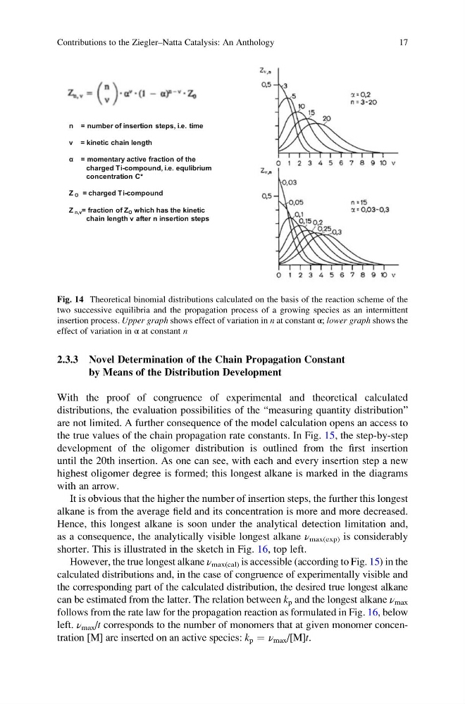
n = number of insertion steps, i.e. time
ν = kinetic chain length
α = momentary active fraction of the
charged Ti-compound, i.e. equlibrium
concentration C*
Z O = charged Ti-compound
Z n,ν = fraction of Z O which has the kinetic
chain length ν after n insertion steps
Fig. 14 Theoretical binomial distributions calculated on the basis of the reaction scheme of the
two successive equilibria and the propagation process of a growing species as an intermittent
insertion process. Upper graph shows effect of variation in n at constant α; lower graph shows the
effect of variation in α at constant n
Contributions to the Ziegler–Natta Catalysis: An Anthology
17
by Means of the Distribution Development
With the proof of congruence of experimental and theoretical calculated
distributions, the evaluation possibilities of the “measuring quantity distribution”
are not limited. A further consequence of the model calculation opens an access to
the true values of the chain propagation rate constants. In Fig. 15, the step-by-step
development of the oligomer distribution is outlined from the first insertion
until the 20th insertion. As one can see, with each and every insertion step a new
highest oligomer degree is formed; this longest alkane is marked in the diagrams
with an arrow.
It is obvious that the higher the number of insertion steps, the further this longest
alkane is from the average field and its concentration is more and more decreased.
Hence, this longest alkane is soon under the analytical detection limitation and,
as a consequence, the analytically visible longest alkane ν max(exp) is considerably
shorter. This is illustrated in the sketch in Fig. 16, top left.
However, the true longest alkane ν max(cal) is accessible (according to Fig. 15) in the
calculated distributions and, in the case of congruence of experimentally visible and
the corresponding part of the calculated distribution, the desired true longest alkane
can be estimated from the latter. The relation between k p and the longest alkane ν max
follows from the rate law for the propagation reaction as formulated in Fig. 16, below
left. ν max /t corresponds to the number of monomers that at given monomer concentration [M] are inserted on an active species: k p ¼ ν max /[M]t.
n = number of insertion steps, i.e. time
ν = kinetic chain length
α = momentary active fraction of the
charged Ti-compound, i.e. equlibrium
concentration C*
Z O = charged Ti-compound
Z n,ν = fraction of Z O which has the kinetic
chain length ν after n insertion steps
Fig. 14 Theoretical binomial distributions calculated on the basis of the reaction scheme of the
two successive equilibria and the propagation process of a growing species as an intermittent
insertion process. Upper graph shows effect of variation in n at constant α; lower graph shows the
effect of variation in α at constant n
Contributions to the Ziegler–Natta Catalysis: An Anthology
17