

62
Z. Amini et al.
Similarly, for two-sided Rayleigh noise, the shrinkage function (3.30), which is
called BiGaussRayMixShrinkL, can be written as:
ˆ
w(k)
1
1 + R( ¯
y(k))
2z 1 (k)
√
2
2 −
σ 2
11 (k)
α 2
+
π
2
1 −
σ 2
11 (k)z 2
1 (k)
α 2
(er f cx(z 1 (k)) − er f cx(−z 1 (k)))
1
α 2 +
1
σ 2
11 (k)
(2 + z 1 (k)
√
πer f cx(−z 1 (k)) − z 1 (k)
√
πer f cx(z 1 (k)))
+
R( ¯
y(k))
1 + R( ¯
y(k))
2z 2 (k)
√
2
2 −
σ 2
21 (k)
α 2
+
π
2
1 −
σ 2
21 (k)z 2
2 (k)
α 2
(er f cx(z 2 (k)) − er f cx(−z 2 (k)))
1
α 2 +
1
σ 2
21 (k)
(2 + z 2 (k)
√
πer f cx(−z 2 (k)) − z 2 (k)
√
πer f cx(z 2 (k)))
(3.38)
where
R( ¯
y(k))
1 − a(k)
a(k)
1 +
σ 2
11 (k)
α 2
1 +
σ 2
12 (k)
α 2
σ 11 (k)σ 12 (k)
1 +
σ 2
21 (k)
α 2
1 +
σ 2
22 (k)
α 2
σ 2i1 (k)σ 22 (k)
exp
−
y 2 (k)
2σ 2
21 (k)
−
y 2
p (k)
2σ 2
22 (k)
exp
−
y 2 (k)
2σ 2
11 (k)
−
y 2
p (k)
2σ 2
12 (k)
×
(2 + z 2 (k)
√
π er f cx(−z 2 (k)) − z 2 (k)
√
πer f cx(z 2 (k)))(2 + z 2 p (k)
√
π er f cx(−z 2 p (k))
(2 + z 1 (k)
√
π er f cx(−z 1 (k)) − z 1 (k)
√
πer f cx(z 1 (k)))(2 + z 1 p (k)
√
π er f cx(−z 1 p (k))
−z 2 p (k)
√
πer f cx(z 2 p (k))
−z 1 p (k)
√
πer f cx(z 1 p (k))
(3.39)
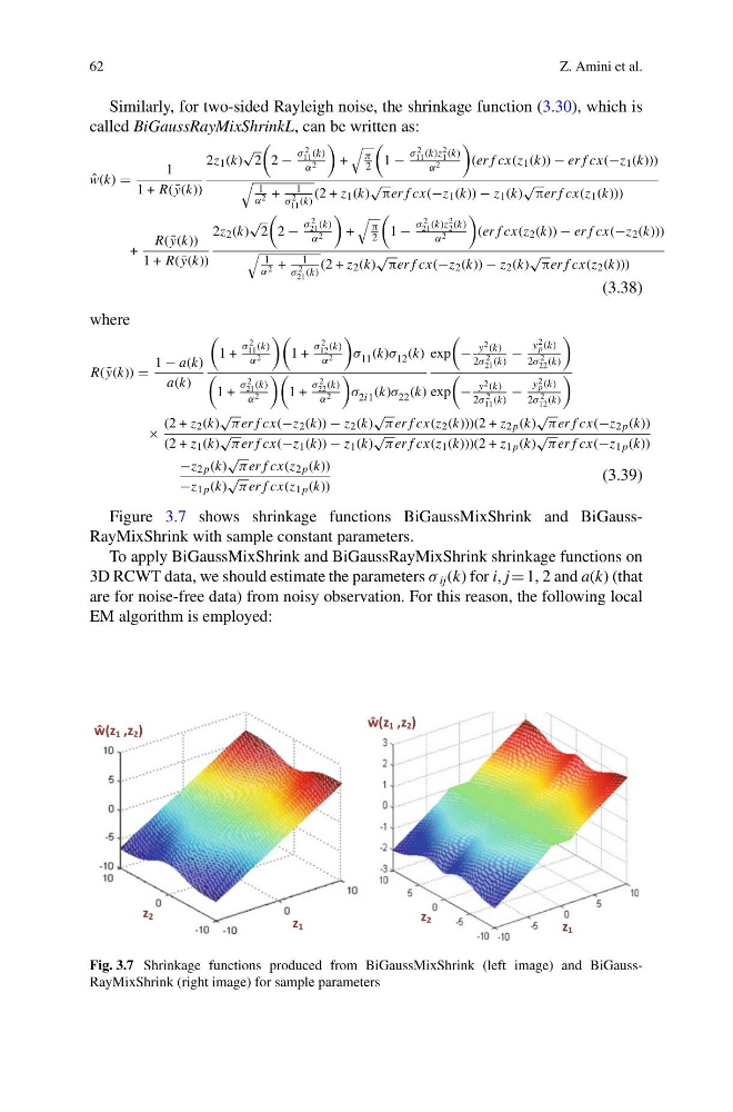
Figure 3.7 shows shrinkage functions BiGaussMixShrink and BiGaussRayMixShrink with sample constant parameters.
To apply BiGaussMixShrink and BiGaussRayMixShrink shrinkage functions on
3D RCWT data, we should estimate the parameters σ ij (k) for i, j 1, 2 and a(k) (that
are for noise-free data) from noisy observation. For this reason, the following local
EM algorithm is employed:
ŵ(z 1 ,z 2 )
z 1
z 2
ŵ(z 1 ,z 2 )
z 2
z 1
Fig. 3.7 Shrinkage functions produced from BiGaussMixShrink (left image) and BiGaussRayMixShrink (right image) for sample parameters
Z. Amini et al.
Similarly, for two-sided Rayleigh noise, the shrinkage function (3.30), which is
called BiGaussRayMixShrinkL, can be written as:
ˆ
w(k)
1
1 + R( ¯
y(k))
2z 1 (k)
√
2
2 −
σ 2
11 (k)
α 2
+
π
2
1 −
σ 2
11 (k)z 2
1 (k)
α 2
(er f cx(z 1 (k)) − er f cx(−z 1 (k)))
1
α 2 +
1
σ 2
11 (k)
(2 + z 1 (k)
√
πer f cx(−z 1 (k)) − z 1 (k)
√
πer f cx(z 1 (k)))
+
R( ¯
y(k))
1 + R( ¯
y(k))
2z 2 (k)
√
2
2 −
σ 2
21 (k)
α 2
+
π
2
1 −
σ 2
21 (k)z 2
2 (k)
α 2
(er f cx(z 2 (k)) − er f cx(−z 2 (k)))
1
α 2 +
1
σ 2
21 (k)
(2 + z 2 (k)
√
πer f cx(−z 2 (k)) − z 2 (k)
√
πer f cx(z 2 (k)))
(3.38)
where
R( ¯
y(k))
1 − a(k)
a(k)
1 +
σ 2
11 (k)
α 2
1 +
σ 2
12 (k)
α 2
σ 11 (k)σ 12 (k)
1 +
σ 2
21 (k)
α 2
1 +
σ 2
22 (k)
α 2
σ 2i1 (k)σ 22 (k)
exp
−
y 2 (k)
2σ 2
21 (k)
−
y 2
p (k)
2σ 2
22 (k)
exp
−
y 2 (k)
2σ 2
11 (k)
−
y 2
p (k)
2σ 2
12 (k)
×
(2 + z 2 (k)
√
π er f cx(−z 2 (k)) − z 2 (k)
√
πer f cx(z 2 (k)))(2 + z 2 p (k)
√
π er f cx(−z 2 p (k))
(2 + z 1 (k)
√
π er f cx(−z 1 (k)) − z 1 (k)
√
πer f cx(z 1 (k)))(2 + z 1 p (k)
√
π er f cx(−z 1 p (k))
−z 2 p (k)
√
πer f cx(z 2 p (k))
−z 1 p (k)
√
πer f cx(z 1 p (k))
(3.39)
Figure 3.7 shows shrinkage functions BiGaussMixShrink and BiGaussRayMixShrink with sample constant parameters.
To apply BiGaussMixShrink and BiGaussRayMixShrink shrinkage functions on
3D RCWT data, we should estimate the parameters σ ij (k) for i, j 1, 2 and a(k) (that
are for noise-free data) from noisy observation. For this reason, the following local
EM algorithm is employed:
ŵ(z 1 ,z 2 )
z 1
z 2
ŵ(z 1 ,z 2 )
z 2
z 1
Fig. 3.7 Shrinkage functions produced from BiGaussMixShrink (left image) and BiGaussRayMixShrink (right image) for sample parameters