

5 Segmentation of OCT Scans Using Probabilistic Graphical Models
127
Optimization with Respect to q b
The previous section derived the terms of the objective function J (q b , q c ). We now
turn to the problem of optimizing J (q b , q c ) with respect to ¯
μ and , the parameters
of q b . Recall that in (5.28) we defined vectors ω 1, j and matrices k, j whose entries
were all depend on ¯
μ and . More dependencies are due to the expectation of p(b)
with respect to q b (5.31) and the entropy of q b (5.32). Inspecting all these terms,
we see that ¯
μ and are independent from each other, so we can optimize them
separately.
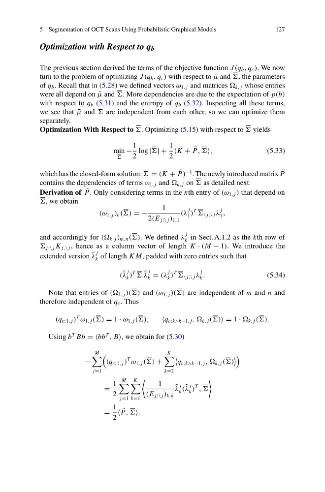
Optimization With Respect to . Optimizing (5.15) with respect to yields
min
−
1
2
log || +
1
2
K + ˜
P, ,
(5.33)
which has the closed-form solution: = (K + ˜
P)
−1 . The newly introduced matrix ˜
P
contains the dependencies of terms ω 1, j and k, j on as detailed next.
Derivation of ˜
P. Only considering terms in the nth entry of (ω 1, j ) that depend on
, we obtain
(ω 1, j ) n () = −
1
2(E j|\ j ) 1,1
(λ
j
1 )
T
\ j,\ j λ
j
1 ,
and accordingly for (( k, j ) m,n (). We defined λ
j
k in Sect. A.1.2 as the kth row of
j|\ j K j,\ j , hence as a column vector of length K · (M − 1). We introduce the
extended version ˜
λ
j
k of length K M, padded with zero entries such that
( ˜
λ
j
k )
T
˜
λ
j
k = (λ
j
k )
T
\ j,\ j λ
j
k .
(5.34)
Note that entries of (( k, j )() and (ω 1, j )() are independent of m and n and
therefore independent of q c . Thus
(q c;1, j )
T
ω 1, j () = 1 · ω 1, j (),
q c;k∧k−1, j , , k, j () = 1 · k, j ().
Using b
T Bb = =bb
T
, B, we obtain for (5.30)
−
M
j=1
(q c;1, j )
T
ω 1, j () +
K
k=2
q c;k∧k−1, j , , k, j ()
=
1
2
M
j=1
K
k=1
1
(E j|\ j ) k,k
˜
λ
j
k ( ˜
λ
j
k )
T
,
=
1
2
˜
P, .
127
Optimization with Respect to q b
The previous section derived the terms of the objective function J (q b , q c ). We now
turn to the problem of optimizing J (q b , q c ) with respect to ¯
μ and , the parameters
of q b . Recall that in (5.28) we defined vectors ω 1, j and matrices k, j whose entries
were all depend on ¯
μ and . More dependencies are due to the expectation of p(b)
with respect to q b (5.31) and the entropy of q b (5.32). Inspecting all these terms,
we see that ¯
μ and are independent from each other, so we can optimize them
separately.
Optimization With Respect to . Optimizing (5.15) with respect to yields
min
−
1
2
log || +
1
2
K + ˜
P, ,
(5.33)
which has the closed-form solution: = (K + ˜
P)
−1 . The newly introduced matrix ˜
P
contains the dependencies of terms ω 1, j and k, j on as detailed next.
Derivation of ˜
P. Only considering terms in the nth entry of (ω 1, j ) that depend on
, we obtain
(ω 1, j ) n () = −
1
2(E j|\ j ) 1,1
(λ
j
1 )
T
\ j,\ j λ
j
1 ,
and accordingly for (( k, j ) m,n (). We defined λ
j
k in Sect. A.1.2 as the kth row of
j|\ j K j,\ j , hence as a column vector of length K · (M − 1). We introduce the
extended version ˜
λ
j
k of length K M, padded with zero entries such that
( ˜
λ
j
k )
T
˜
λ
j
k = (λ
j
k )
T
\ j,\ j λ
j
k .
(5.34)
Note that entries of (( k, j )() and (ω 1, j )() are independent of m and n and
therefore independent of q c . Thus
(q c;1, j )
T
ω 1, j () = 1 · ω 1, j (),
q c;k∧k−1, j , , k, j () = 1 · k, j ().
Using b
T Bb = =bb
T
, B, we obtain for (5.30)
−
M
j=1
(q c;1, j )
T
ω 1, j () +
K
k=2
q c;k∧k−1, j , , k, j ()
=
1
2
M
j=1
K
k=1
1
(E j|\ j ) k,k
˜
λ
j
k ( ˜
λ
j
k )
T
,
=
1
2
˜
P, .