

5 Segmentation of OCT Scans Using Probabilistic Graphical Models
107
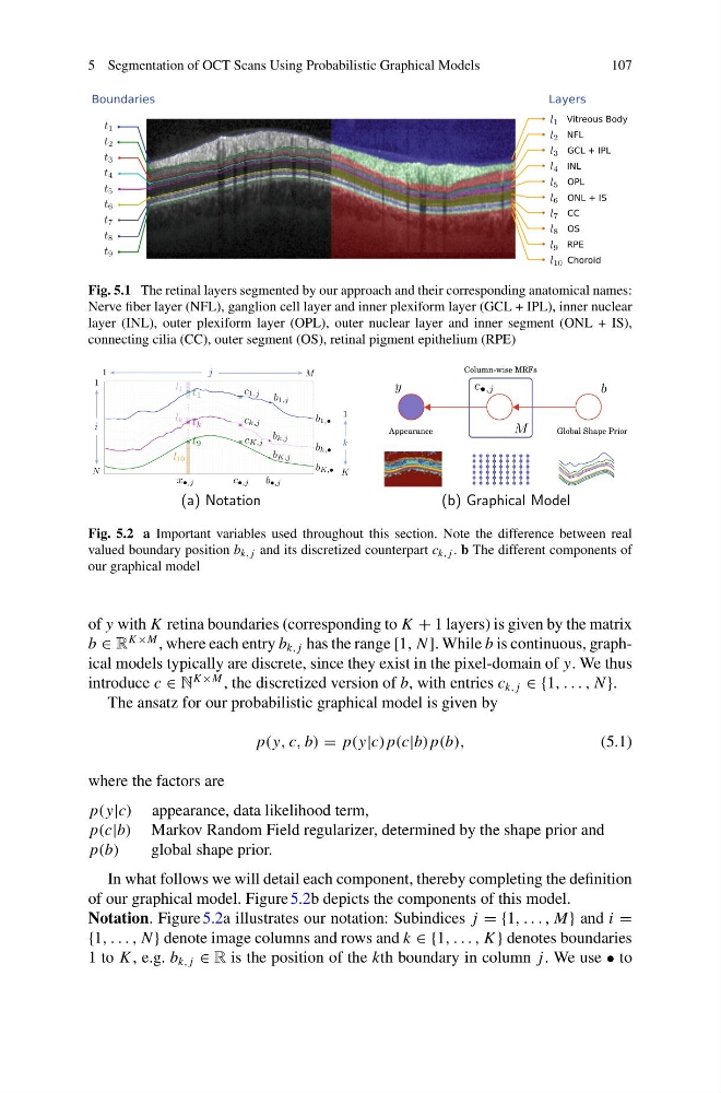
Fig. 5.1 The retinal layers segmented by our approach and their corresponding anatomical names:
Nerve fiber layer (NFL), ganglion cell layer and inner plexiform layer (GCL + IPL), inner nuclear
layer (INL), outer plexiform layer (OPL), outer nuclear layer and inner segment (ONL + IS),
connecting cilia (CC), outer segment (OS), retinal pigment epithelium (RPE)
Fig. 5.2 a Important variables used throughout this section. Note the difference between real
valued boundary position b k, j and its discretized counterpart c k, j . b The different components of
our graphical model
of y with K retina boundaries (corresponding to K + 1 layers) is given by the matrix
b ∈ R
K ×M , where each entry b k, j has the range [1, N ]. While b is continuous, graphical models typically are discrete, since they exist in the pixel-domain of y. We thus
introduce c ∈ N
K ×M , the discretized version of b, with entries c k, j ∈ {1, . . . , N }.
The ansatz for our probabilistic graphical model is given by
p(y, c, b) = p(y|c) p(c|b) p(b),
(5.1)
where the factors are
p(y|c) appearance, data likelihood term,
p(c|b) Markov Random Field regularizer, determined by the shape prior and
p(b)
global shape prior.
In what follows we will detail each component, thereby completing the definition
of our graphical model. Figure 5.2b depicts the components of this model.
Notation. Figure 5.2a illustrates our notation: Subindices j = {1, . . . , M} and i =
{1, . . . , N } denote image columns and rows and k ∈ {1, . . . , K } denotes boundaries
1 to K , e.g. b k, j ∈ R is the position of the kth boundary in column j. We use • to
107
Fig. 5.1 The retinal layers segmented by our approach and their corresponding anatomical names:
Nerve fiber layer (NFL), ganglion cell layer and inner plexiform layer (GCL + IPL), inner nuclear
layer (INL), outer plexiform layer (OPL), outer nuclear layer and inner segment (ONL + IS),
connecting cilia (CC), outer segment (OS), retinal pigment epithelium (RPE)
Fig. 5.2 a Important variables used throughout this section. Note the difference between real
valued boundary position b k, j and its discretized counterpart c k, j . b The different components of
our graphical model
of y with K retina boundaries (corresponding to K + 1 layers) is given by the matrix
b ∈ R
K ×M , where each entry b k, j has the range [1, N ]. While b is continuous, graphical models typically are discrete, since they exist in the pixel-domain of y. We thus
introduce c ∈ N
K ×M , the discretized version of b, with entries c k, j ∈ {1, . . . , N }.
The ansatz for our probabilistic graphical model is given by
p(y, c, b) = p(y|c) p(c|b) p(b),
(5.1)
where the factors are
p(y|c) appearance, data likelihood term,
p(c|b) Markov Random Field regularizer, determined by the shape prior and
p(b)
global shape prior.
In what follows we will detail each component, thereby completing the definition
of our graphical model. Figure 5.2b depicts the components of this model.
Notation. Figure 5.2a illustrates our notation: Subindices j = {1, . . . , M} and i =
{1, . . . , N } denote image columns and rows and k ∈ {1, . . . , K } denotes boundaries
1 to K , e.g. b k, j ∈ R is the position of the kth boundary in column j. We use • to