

96
L. Fang and S. Li
3D Adaptive Sparse Representation
Input: Offline: 1 ,..., U
x
x training patches extracted from the less noisy training images;
Online:
1 ,...,
T
i
i
x
x nearby patches extracted from the position i of the nearby slices.
A) Offline Structural Dictionary Construction:
1: Cluster the training patches 1 ,..., U
x
x into H groups using the k-means approach.
2: For each cluster, compute one centroid h
c and learn one structural sub-dictionary
structural
h
D
.
B) Online 3D Adaptive Sparse Decomposition:
1: Select the fitted sub-dictionaries
structural
ˆt
i
h
D
for the nearby patches
1 ,...,
T
i
i
x
x in Eq. (4-18).
2: Based on the selected sub-dictionaries, divide the nearby patches into two groups: Similar and
Different.
3: If nearby patches are similar, obtain their sparse vectors { }
sim,
1
ˆ
T
t
i t =
α
by jointly decomposing
nearby patches on the same atoms from the commonly selected sub-dictionary in Eq. (4-19).
4: Further divide the sparse vectors { }
sim,
1
ˆ
T
t
i t =
α
into two groups: very similar s,
v i
α and not very
similar { }
nvs,
1
ˆ
T
t
i t =
α
in Eq. (4-20).
5: If nearby patches are different, obtain their sparse vectors { }
dif ,
1
ˆ
T
t
i t =
α
by separately
decomposing nearby patches on different sub-dictionaries in Eq. (4-21).
Output: { }
dif ,
1
ˆ
T
t
i t =
α
if the nearby patches are different; { }
nvs,
1
ˆ
T
t
i t =
α
if the nearby slices are not very
similar; s,
v i
α
if the nearby patches are very similar.
Fig. 4.15 3D adaptive sparse representation algorithm
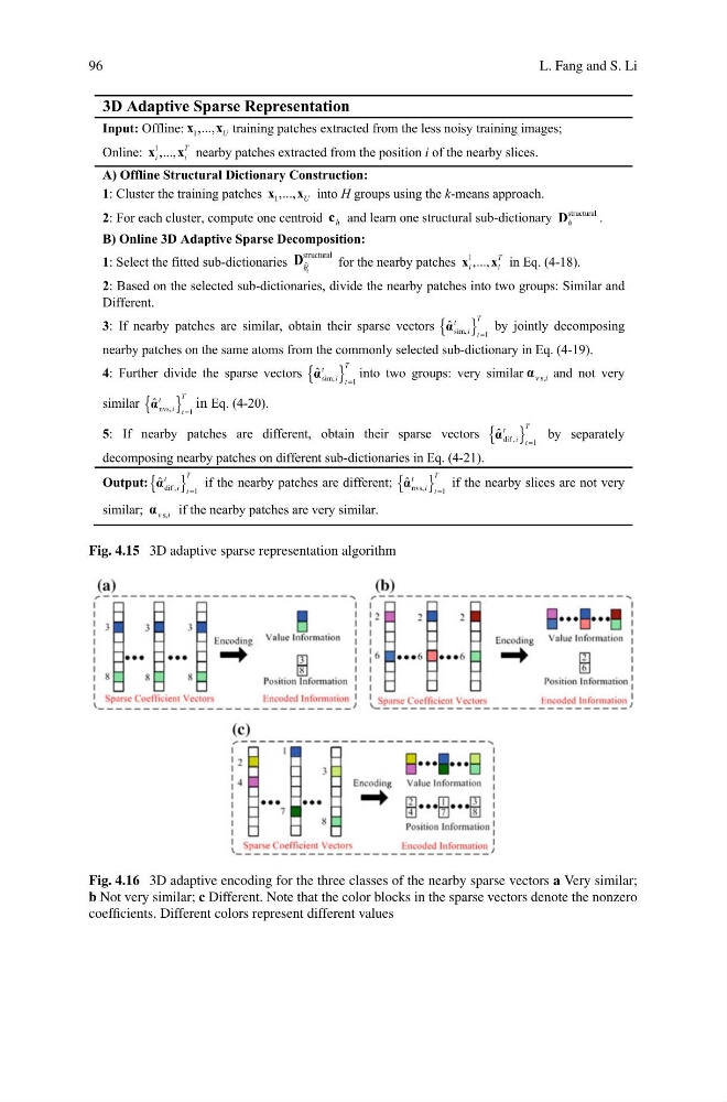
Fig. 4.16 3D adaptive encoding for the three classes of the nearby sparse vectors a Very similar;
b Not very similar; c Different. Note that the color blocks in the sparse vectors denote the nonzero
coefficients. Different colors represent different values
L. Fang and S. Li
3D Adaptive Sparse Representation
Input: Offline: 1 ,..., U
x
x training patches extracted from the less noisy training images;
Online:
1 ,...,
T
i
i
x
x nearby patches extracted from the position i of the nearby slices.
A) Offline Structural Dictionary Construction:
1: Cluster the training patches 1 ,..., U
x
x into H groups using the k-means approach.
2: For each cluster, compute one centroid h
c and learn one structural sub-dictionary
structural
h
D
.
B) Online 3D Adaptive Sparse Decomposition:
1: Select the fitted sub-dictionaries
structural
ˆt
i
h
D
for the nearby patches
1 ,...,
T
i
i
x
x in Eq. (4-18).
2: Based on the selected sub-dictionaries, divide the nearby patches into two groups: Similar and
Different.
3: If nearby patches are similar, obtain their sparse vectors { }
sim,
1
ˆ
T
t
i t =
α
by jointly decomposing
nearby patches on the same atoms from the commonly selected sub-dictionary in Eq. (4-19).
4: Further divide the sparse vectors { }
sim,
1
ˆ
T
t
i t =
α
into two groups: very similar s,
v i
α and not very
similar { }
nvs,
1
ˆ
T
t
i t =
α
in Eq. (4-20).
5: If nearby patches are different, obtain their sparse vectors { }
dif ,
1
ˆ
T
t
i t =
α
by separately
decomposing nearby patches on different sub-dictionaries in Eq. (4-21).
Output: { }
dif ,
1
ˆ
T
t
i t =
α
if the nearby patches are different; { }
nvs,
1
ˆ
T
t
i t =
α
if the nearby slices are not very
similar; s,
v i
α
if the nearby patches are very similar.
Fig. 4.15 3D adaptive sparse representation algorithm
Fig. 4.16 3D adaptive encoding for the three classes of the nearby sparse vectors a Very similar;
b Not very similar; c Different. Note that the color blocks in the sparse vectors denote the nonzero
coefficients. Different colors represent different values