

270
X. Liu et al.
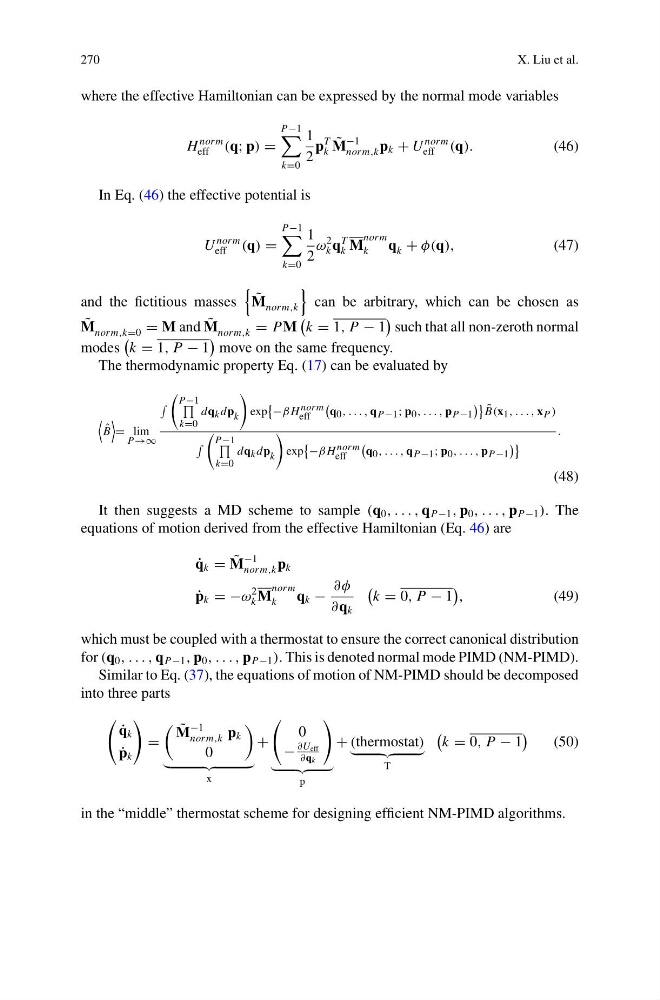
where the effective Hamiltonian can be expressed by the normal mode variables
H
norm
eff (q; p) =
P−1
k=0
1
2
p
T
k
˜
M
−1
norm,k p k + U
norm
eff (q).
(46)
In Eq. (46) the effective potential is
U
norm
eff (q) =
P−1
k=0
1
2
ω
2
k q
T
k M
norm
k
q k + φ(q),
(47)
and the fictitious masses
˜
M norm,k
can be arbitrary, which can be chosen as
˜
M norm,k=0 = M and ˜
M norm,k = PM
k = 1, P − 1
such that all non-zeroth normal
modes
k = 1, P − 1
move on the same frequency.
The thermodynamic property Eq. (17) can be evaluated by
ˆ
B
= lim
P→∞
P−1
k=0
dq k dp k
exp
−β H norm
eff
q 0 , . . . , q P−1 ; p 0 , . . . , p P−1
˜
B(x 1 , . . . , x P )
P−1
k=0
dq k dp k
exp
−β H norm
eff
q 0 , . . . , q P−1 ; p 0 , . . . , p P−1
.
(48)
It then suggests a MD scheme to sample (q 0 , . . . , q P−1 , p 0 , . . . , p P−1 ). The
equations of motion derived from the effective Hamiltonian (Eq. 46) are
˙
q k = ˜
M
−1
norm,k p k
˙
p k = −ω
2
k M
norm
k
q k −
∂φ
∂q k
k = 0, P − 1
,
(49)
which must be coupled with a thermostat to ensure the correct canonical distribution
for (q 0 , . . . , q P−1 , p 0 , . . . , p P−1 ). This is denoted normal mode PIMD (NM-PIMD).
Similar to Eq. (37), the equations of motion of NM-PIMD should be decomposed
into three parts
˙
q k
˙
p k
=
˜
M
−1
norm,k p k
0
x
+
0
−
∂U eff
∂q k
p
+ (thermostat)
T
k = 0, P − 1
(50)
in the “middle” thermostat scheme for designing efficient NM-PIMD algorithms.
X. Liu et al.
where the effective Hamiltonian can be expressed by the normal mode variables
H
norm
eff (q; p) =
P−1
k=0
1
2
p
T
k
˜
M
−1
norm,k p k + U
norm
eff (q).
(46)
In Eq. (46) the effective potential is
U
norm
eff (q) =
P−1
k=0
1
2
ω
2
k q
T
k M
norm
k
q k + φ(q),
(47)
and the fictitious masses
˜
M norm,k
can be arbitrary, which can be chosen as
˜
M norm,k=0 = M and ˜
M norm,k = PM
k = 1, P − 1
such that all non-zeroth normal
modes
k = 1, P − 1
move on the same frequency.
The thermodynamic property Eq. (17) can be evaluated by
ˆ
B
= lim
P→∞
P−1
k=0
dq k dp k
exp
−β H norm
eff
q 0 , . . . , q P−1 ; p 0 , . . . , p P−1
˜
B(x 1 , . . . , x P )
P−1
k=0
dq k dp k
exp
−β H norm
eff
q 0 , . . . , q P−1 ; p 0 , . . . , p P−1
.
(48)
It then suggests a MD scheme to sample (q 0 , . . . , q P−1 , p 0 , . . . , p P−1 ). The
equations of motion derived from the effective Hamiltonian (Eq. 46) are
˙
q k = ˜
M
−1
norm,k p k
˙
p k = −ω
2
k M
norm
k
q k −
∂φ
∂q k
k = 0, P − 1
,
(49)
which must be coupled with a thermostat to ensure the correct canonical distribution
for (q 0 , . . . , q P−1 , p 0 , . . . , p P−1 ). This is denoted normal mode PIMD (NM-PIMD).
Similar to Eq. (37), the equations of motion of NM-PIMD should be decomposed
into three parts
˙
q k
˙
p k
=
˜
M
−1
norm,k p k
0
x
+
0
−
∂U eff
∂q k
p
+ (thermostat)
T
k = 0, P − 1
(50)
in the “middle” thermostat scheme for designing efficient NM-PIMD algorithms.