

Efficient “Middle” Thermostat Scheme …
263
0.0
0.5
1.0
1.5
2.0
-2000
-1800
-1600
-1400
-1200
-1000
0.0
0.5
1.0
1.5
2.0
460
480
500
520
540
560
580
600
620
(a)
(b)
Potential energy (kcal/mol)
Time interval (fs)
LF-Middle
VV-Middle
Side
Old
(b)
LF-Middle
VV-Middle
Side
Old
Time interval (fs)
Kinetic energy (kcal/mol)
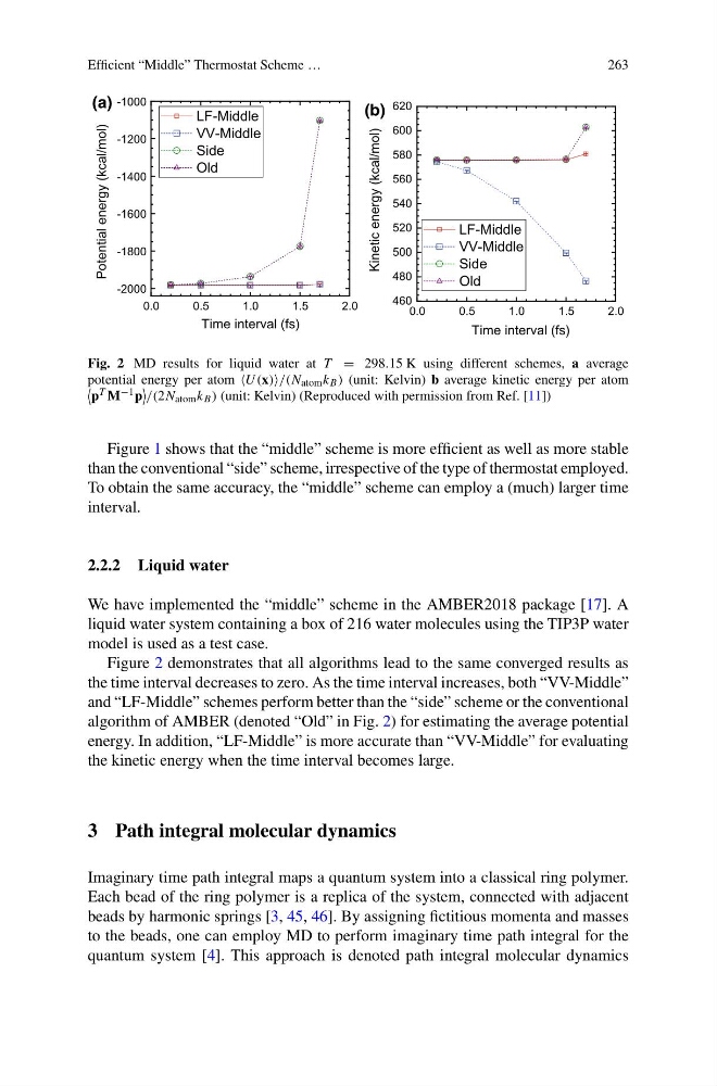
Fig. 2 MD results for liquid water at T = 298.15 K using different schemes, a average
potential energy per atom U (x)/(N atom k B ) (unit: Kelvin) b average kinetic energy per atom
p T M −1 p
/(2N atom k B ) (unit: Kelvin) (Reproduced with permission from Ref. [11])
Figure 1 shows that the “middle” scheme is more efficient as well as more stable
than the conventional “side” scheme, irrespective of the type of thermostat employed.
To obtain the same accuracy, the “middle” scheme can employ a (much) larger time
interval.
2.2.2 Liquid water
We have implemented the “middle” scheme in the AMBER2018 package [17]. A
liquid water system containing a box of 216 water molecules using the TIP3P water
model is used as a test case.
Figure 2 demonstrates that all algorithms lead to the same converged results as
the time interval decreases to zero. As the time interval increases, both “VV-Middle”
and “LF-Middle” schemes perform better than the “side” scheme or the conventional
algorithm of AMBER (denoted “Old” in Fig. 2) for estimating the average potential
energy. In addition, “LF-Middle” is more accurate than “VV-Middle” for evaluating
the kinetic energy when the time interval becomes large.
3 Path integral molecular dynamics
Imaginary time path integral maps a quantum system into a classical ring polymer.
Each bead of the ring polymer is a replica of the system, connected with adjacent
beads by harmonic springs [3, 45, 46]. By assigning fictitious momenta and masses
to the beads, one can employ MD to perform imaginary time path integral for the
quantum system [4]. This approach is denoted path integral molecular dynamics
263
0.0
0.5
1.0
1.5
2.0
-2000
-1800
-1600
-1400
-1200
-1000
0.0
0.5
1.0
1.5
2.0
460
480
500
520
540
560
580
600
620
(a)
(b)
Potential energy (kcal/mol)
Time interval (fs)
LF-Middle
VV-Middle
Side
Old
(b)
LF-Middle
VV-Middle
Side
Old
Time interval (fs)
Kinetic energy (kcal/mol)
Fig. 2 MD results for liquid water at T = 298.15 K using different schemes, a average
potential energy per atom U (x)/(N atom k B ) (unit: Kelvin) b average kinetic energy per atom
p T M −1 p
/(2N atom k B ) (unit: Kelvin) (Reproduced with permission from Ref. [11])
Figure 1 shows that the “middle” scheme is more efficient as well as more stable
than the conventional “side” scheme, irrespective of the type of thermostat employed.
To obtain the same accuracy, the “middle” scheme can employ a (much) larger time
interval.
2.2.2 Liquid water
We have implemented the “middle” scheme in the AMBER2018 package [17]. A
liquid water system containing a box of 216 water molecules using the TIP3P water
model is used as a test case.
Figure 2 demonstrates that all algorithms lead to the same converged results as
the time interval decreases to zero. As the time interval increases, both “VV-Middle”
and “LF-Middle” schemes perform better than the “side” scheme or the conventional
algorithm of AMBER (denoted “Old” in Fig. 2) for estimating the average potential
energy. In addition, “LF-Middle” is more accurate than “VV-Middle” for evaluating
the kinetic energy when the time interval becomes large.
3 Path integral molecular dynamics
Imaginary time path integral maps a quantum system into a classical ring polymer.
Each bead of the ring polymer is a replica of the system, connected with adjacent
beads by harmonic springs [3, 45, 46]. By assigning fictitious momenta and masses
to the beads, one can employ MD to perform imaginary time path integral for the
quantum system [4]. This approach is denoted path integral molecular dynamics