

84 Beam-based Correction and Optimization for Accelerators
x (mm)
-5
0
5
uncorrected
s (m)
0
50
100
150
200
x (mm)
-2
0
2
corrected w/ 6 SVs
corrected w/ 56 SVs
Horizontal corrector
0
10
20
30
40
50
60
∆θ (mrad)
-0.2
0
0.2
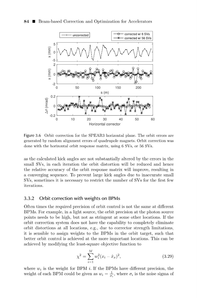
Figure 3.6 Orbit correction for the SPEAR3 horizontal plane. The orbit errors are
generated by random alignment errors of quadrupole magnets. Orbit correction was
done with the horizontal orbit response matrix, using 6 SVs, or 56 SVs.
as the calculated kick angles are not substantially altered by the errors in the
small SVs, in each iteration the orbit distortion will be reduced and hence
the relative accuracy of the orbit response matrix will improve, resulting in
a converging sequence. To prevent large kick angles due to inaccurate small
SVs, sometimes it is necessary to restrict the number of SVs for the first few
iterations.
3.3.2 Orbit correction with weights on BPMs
Often times the required precision of orbit control is not the same at different
BPMs. For example, in a light source, the orbit precision at the photon source
points needs to be high, but not as stringent at some other locations. If the
orbit correction system does not have the capability to completely eliminate
orbit distortions at all locations, e.g., due to corrector strength limitations,
it is sensible to assign weights to the BPMs in the orbit target, such that
better orbit control is achieved at the more important locations. This can be
achieved by modifying the least-square objective function to
χ
2 =
M
i=1
w
2
i (x i − ˆ
x x )
2 ,
(3.29)
where w i is the weight for BPM i. If the BPMs have different precision, the
weight of each BPM could be given as w i =
1
σi , where σ i is the noise sigma of
x (mm)
-5
0
5
uncorrected
s (m)
0
50
100
150
200
x (mm)
-2
0
2
corrected w/ 6 SVs
corrected w/ 56 SVs
Horizontal corrector
0
10
20
30
40
50
60
∆θ (mrad)
-0.2
0
0.2
Figure 3.6 Orbit correction for the SPEAR3 horizontal plane. The orbit errors are
generated by random alignment errors of quadrupole magnets. Orbit correction was
done with the horizontal orbit response matrix, using 6 SVs, or 56 SVs.
as the calculated kick angles are not substantially altered by the errors in the
small SVs, in each iteration the orbit distortion will be reduced and hence
the relative accuracy of the orbit response matrix will improve, resulting in
a converging sequence. To prevent large kick angles due to inaccurate small
SVs, sometimes it is necessary to restrict the number of SVs for the first few
iterations.
3.3.2 Orbit correction with weights on BPMs
Often times the required precision of orbit control is not the same at different
BPMs. For example, in a light source, the orbit precision at the photon source
points needs to be high, but not as stringent at some other locations. If the
orbit correction system does not have the capability to completely eliminate
orbit distortions at all locations, e.g., due to corrector strength limitations,
it is sensible to assign weights to the BPMs in the orbit target, such that
better orbit control is achieved at the more important locations. This can be
achieved by modifying the least-square objective function to
χ
2 =
M
i=1
w
2
i (x i − ˆ
x x )
2 ,
(3.29)
where w i is the weight for BPM i. If the BPMs have different precision, the
weight of each BPM could be given as w i =
1
σi , where σ i is the noise sigma of