

Beam dynamics topics 61
L/2
L/2
0
1
− 1
+
2
drift
kick drift
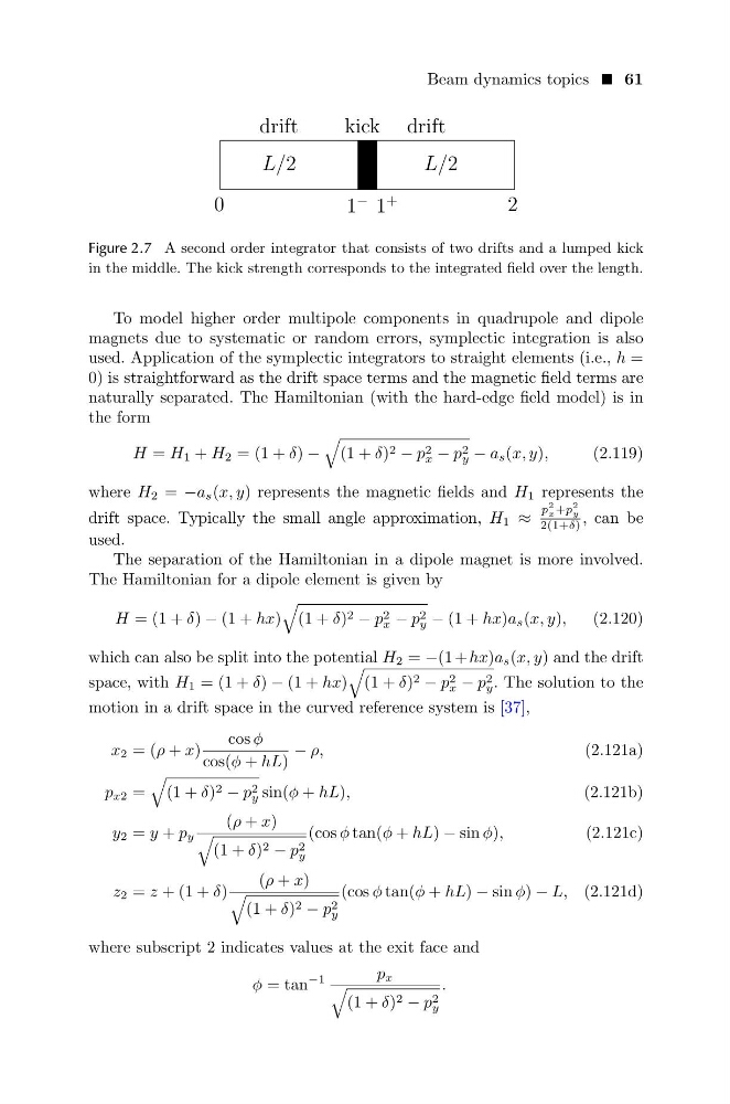
Figure 2.7 A second order integrator that consists of two drifts and a lumped kick
in the middle. The kick strength corresponds to the integrated field over the length.
To model higher order multipole components in quadrupole and dipole
magnets due to systematic or random errors, symplectic integration is also
used. Application of the symplectic integrators to straight elements (i.e., h =
0) is straightforward as the drift space terms and the magnetic field terms are
naturally separated. The Hamiltonian (with the hard-edge field model) is in
the form
H = H 1 + H 2 = (1 + δ) −
(1 + δ) 2 − p 2
x − p 2
y − a s (x, y),
(2.119)
where H 2 = −a s (x, y) represents the magnetic fields and H 1 represents the
drift space. Typically the small angle approximation, H 1 ≈
p
2
x +p
2
y
2(1+δ) , can be
used.
The separation of the Hamiltonian in a dipole magnet is more involved.
The Hamiltonian for a dipole element is given by
H = (1 + δ) − (1 + hx)
(1 + δ) 2 − p 2
x − p 2
y − (1 + hx)a s (x, y),
(2.120)
which can also be split into the potential H 2 = −(1 + hx)a s (x, y) and the drift
space, with H 1 = (1 + δ) − (1 + hx)
(1 + δ) 2 − p 2
x − p 2
y . The solution to the
motion in a drift space in the curved reference system is [37],
x 2 = (ρ + x)
cos φ
cos(φ + hL)
− ρ,
(2.121a)
p x2 =
(1 + δ) 2 − p 2
y sin(φ + hL),
(2.121b)
y 2 = y + p y
(ρ + x)
(1 + δ) 2 − p 2
y
(cos φ tan(φ + hL) − sin φ),
(2.121c)
z 2 = z + (1 + δ)
(ρ + x)
(1 + δ) 2 − p 2
y
(cos φ tan(φ + hL) − sin φ) − L, (2.121d)
where subscript 2 indicates values at the exit face and
φ = tan
−1
p x
(1 + δ) 2 − p 2
y
.
L/2
L/2
0
1
− 1
+
2
drift
kick drift
Figure 2.7 A second order integrator that consists of two drifts and a lumped kick
in the middle. The kick strength corresponds to the integrated field over the length.
To model higher order multipole components in quadrupole and dipole
magnets due to systematic or random errors, symplectic integration is also
used. Application of the symplectic integrators to straight elements (i.e., h =
0) is straightforward as the drift space terms and the magnetic field terms are
naturally separated. The Hamiltonian (with the hard-edge field model) is in
the form
H = H 1 + H 2 = (1 + δ) −
(1 + δ) 2 − p 2
x − p 2
y − a s (x, y),
(2.119)
where H 2 = −a s (x, y) represents the magnetic fields and H 1 represents the
drift space. Typically the small angle approximation, H 1 ≈
p
2
x +p
2
y
2(1+δ) , can be
used.
The separation of the Hamiltonian in a dipole magnet is more involved.
The Hamiltonian for a dipole element is given by
H = (1 + δ) − (1 + hx)
(1 + δ) 2 − p 2
x − p 2
y − (1 + hx)a s (x, y),
(2.120)
which can also be split into the potential H 2 = −(1 + hx)a s (x, y) and the drift
space, with H 1 = (1 + δ) − (1 + hx)
(1 + δ) 2 − p 2
x − p 2
y . The solution to the
motion in a drift space in the curved reference system is [37],
x 2 = (ρ + x)
cos φ
cos(φ + hL)
− ρ,
(2.121a)
p x2 =
(1 + δ) 2 − p 2
y sin(φ + hL),
(2.121b)
y 2 = y + p y
(ρ + x)
(1 + δ) 2 − p 2
y
(cos φ tan(φ + hL) − sin φ),
(2.121c)
z 2 = z + (1 + δ)
(ρ + x)
(1 + δ) 2 − p 2
y
(cos φ tan(φ + hL) − sin φ) − L, (2.121d)
where subscript 2 indicates values at the exit face and
φ = tan
−1
p x
(1 + δ) 2 − p 2
y
.