

Basics of beam dynamics 21
(a)
y
y
′
Drift:
β = β0 − 2α0s + γ0s
2
α = α0 − γ0s
(b)
y
y
′
Thin QF:
β = β0,
α = α0 +
β0
f
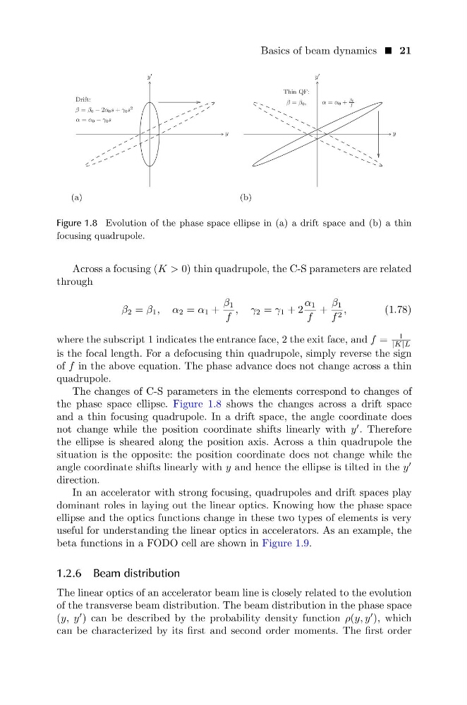
Figure 1.8 Evolution of the phase space ellipse in (a) a drift space and (b) a thin
focusing quadrupole.
Across a focusing (K > 0) thin quadrupole, the C-S parameters are related
through
β 2 = β 1 , α 2 = α 1 +
β 1
f
, γ 2 = γ 1 + 2
α 1
f
+
β 1
f 2 ,
(1.78)
where the subscript 1 indicates the entrance face, 2 the exit face, and f =
1
|K|L
is the focal length. For a defocusing thin quadrupole, simply reverse the sign
of f in the above equation. The phase advance does not change across a thin
quadrupole.
The changes of C-S parameters in the elements correspond to changes of
the phase space ellipse. Figure 1.8 shows the changes across a drift space
and a thin focusing quadrupole. In a drift space, the angle coordinate does
not change while the position coordinate shifts linearly with y
. Therefore
the ellipse is sheared along the position axis. Across a thin quadrupole the
situation is the opposite: the position coordinate does not change while the
angle coordinate shifts linearly with y and hence the ellipse is tilted in the y
direction.
In an accelerator with strong focusing, quadrupoles and drift spaces play
dominant roles in laying out the linear optics. Knowing how the phase space
ellipse and the optics functions change in these two types of elements is very
useful for understanding the linear optics in accelerators. As an example, the
beta functions in a FODO cell are shown in Figure 1.9.
1.2.6 Beam distribution
The linear optics of an accelerator beam line is closely related to the evolution
of the transverse beam distribution. The beam distribution in the phase space
(y, y
) can be described by the probability density function ρ(y, y
), which
can be characterized by its first and second order moments. The first order
(a)
y
y
′
Drift:
β = β0 − 2α0s + γ0s
2
α = α0 − γ0s
(b)
y
y
′
Thin QF:
β = β0,
α = α0 +
β0
f
Figure 1.8 Evolution of the phase space ellipse in (a) a drift space and (b) a thin
focusing quadrupole.
Across a focusing (K > 0) thin quadrupole, the C-S parameters are related
through
β 2 = β 1 , α 2 = α 1 +
β 1
f
, γ 2 = γ 1 + 2
α 1
f
+
β 1
f 2 ,
(1.78)
where the subscript 1 indicates the entrance face, 2 the exit face, and f =
1
|K|L
is the focal length. For a defocusing thin quadrupole, simply reverse the sign
of f in the above equation. The phase advance does not change across a thin
quadrupole.
The changes of C-S parameters in the elements correspond to changes of
the phase space ellipse. Figure 1.8 shows the changes across a drift space
and a thin focusing quadrupole. In a drift space, the angle coordinate does
not change while the position coordinate shifts linearly with y
. Therefore
the ellipse is sheared along the position axis. Across a thin quadrupole the
situation is the opposite: the position coordinate does not change while the
angle coordinate shifts linearly with y and hence the ellipse is tilted in the y
direction.
In an accelerator with strong focusing, quadrupoles and drift spaces play
dominant roles in laying out the linear optics. Knowing how the phase space
ellipse and the optics functions change in these two types of elements is very
useful for understanding the linear optics in accelerators. As an example, the
beta functions in a FODO cell are shown in Figure 1.9.
1.2.6 Beam distribution
The linear optics of an accelerator beam line is closely related to the evolution
of the transverse beam distribution. The beam distribution in the phase space
(y, y
) can be described by the probability density function ρ(y, y
), which
can be characterized by its first and second order moments. The first order