

Basics of beam dynamics 13
(a)
s
x
f
(b)
s
y
f
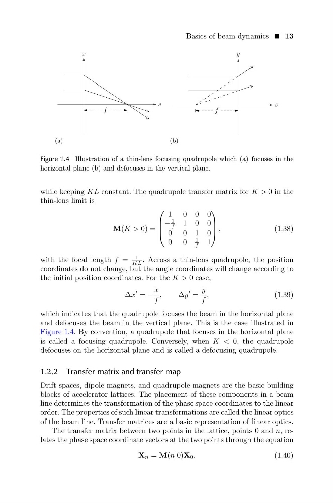
Figure 1.4 Illustration of a thin-lens focusing quadrupole which (a) focuses in the
horizontal plane (b) and defocuses in the vertical plane.
while keeping KL constant. The quadrupole transfer matrix for K > 0 in the
thin-lens limit is
M(K > 0) =
1 0 0 0
−
1
f
1 0 0
0 0 1 0
0 0
1
f
1
,
(1.38)
with the focal length f =
1
KL . Across a thin-lens quadrupole, the position
coordinates do not change, but the angle coordinates will change according to
the initial position coordinates. For the K > 0 case,
∆x
= −
x
f
,
∆y
=
y
f
,
(1.39)
which indicates that the quadrupole focuses the beam in the horizontal plane
and defocuses the beam in the vertical plane. This is the case illustrated in
Figure 1.4. By convention, a quadrupole that focuses in the horizontal plane
is called a focusing quadrupole. Conversely, when K < 0, the quadrupole
defocuses on the horizontal plane and is called a defocusing quadrupole.
1.2.2 Transfer matrix and transfer map
Drift spaces, dipole magnets, and quadrupole magnets are the basic building
blocks of accelerator lattices. The placement of these components in a beam
line determines the transformation of the phase space coordinates to the linear
order. The properties of such linear transformations are called the linear optics
of the beam line. Transfer matrices are a basic representation of linear optics.
The transfer matrix between two points in the lattice, points 0 and n, relates the phase space coordinate vectors at the two points through the equation
X n = M(n|0)X 0 .
(1.40)
(a)
s
x
f
(b)
s
y
f
Figure 1.4 Illustration of a thin-lens focusing quadrupole which (a) focuses in the
horizontal plane (b) and defocuses in the vertical plane.
while keeping KL constant. The quadrupole transfer matrix for K > 0 in the
thin-lens limit is
M(K > 0) =
1 0 0 0
−
1
f
1 0 0
0 0 1 0
0 0
1
f
1
,
(1.38)
with the focal length f =
1
KL . Across a thin-lens quadrupole, the position
coordinates do not change, but the angle coordinates will change according to
the initial position coordinates. For the K > 0 case,
∆x
= −
x
f
,
∆y
=
y
f
,
(1.39)
which indicates that the quadrupole focuses the beam in the horizontal plane
and defocuses the beam in the vertical plane. This is the case illustrated in
Figure 1.4. By convention, a quadrupole that focuses in the horizontal plane
is called a focusing quadrupole. Conversely, when K < 0, the quadrupole
defocuses on the horizontal plane and is called a defocusing quadrupole.
1.2.2 Transfer matrix and transfer map
Drift spaces, dipole magnets, and quadrupole magnets are the basic building
blocks of accelerator lattices. The placement of these components in a beam
line determines the transformation of the phase space coordinates to the linear
order. The properties of such linear transformations are called the linear optics
of the beam line. Transfer matrices are a basic representation of linear optics.
The transfer matrix between two points in the lattice, points 0 and n, relates the phase space coordinate vectors at the two points through the equation
X n = M(n|0)X 0 .
(1.40)