

Online optimization algorithms 191
0
2
4
6
8
10
x
-2
-1
0
1
2
f(x)
Bessel J 0 (x)
sample
(x)
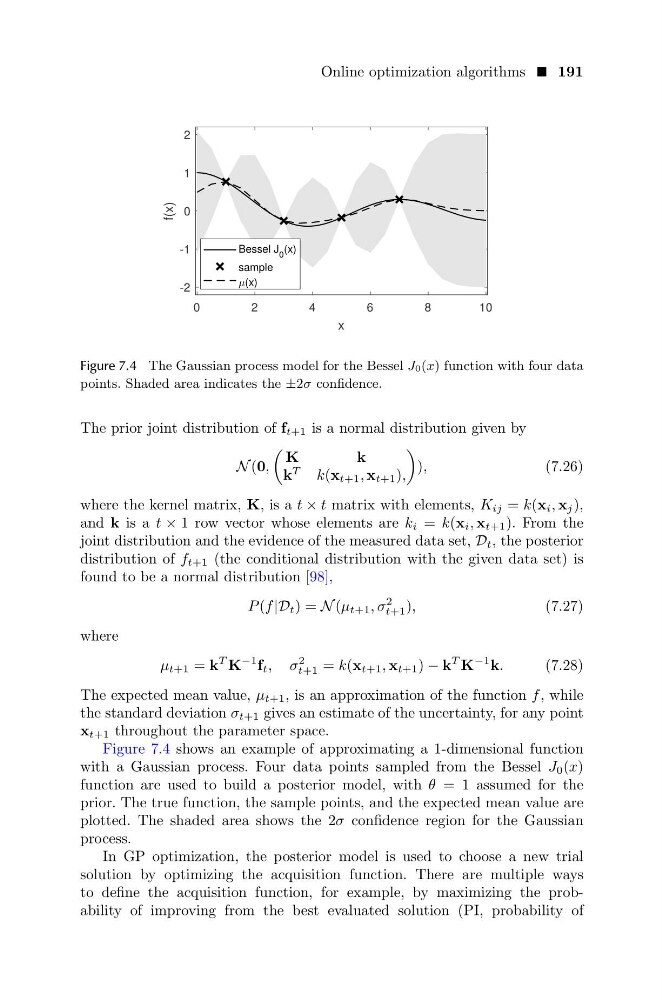
Figure 7.4 The Gaussian process model for the Bessel J0(x) function with four data
points. Shaded area indicates the ±2σ confidence.
The prior joint distribution of f t+1 is a normal distribution given by
N (0,
K
k
k
T
k(x t+1 , x t+1 ),
),
(7.26)
where the kernel matrix, K, is a t × t matrix with elements, K ij = k(x i , x j ),
and k is a t × 1 row vector whose elements are k i = k(x i , x t+1 ). From the
joint distribution and the evidence of the measured data set, D t , the posterior
distribution of f t+1 (the conditional distribution with the given data set) is
found to be a normal distribution [98],
P (f |D t ) = N (µ t+1 , σ
2
t+1 ),
(7.27)
where
µ t+1 = k
T K
−1 f t , σ
2
t+1 = k(x t+1 , x t+1 ) − k
T K
−1 k.
(7.28)
The expected mean value, µ t+1 , is an approximation of the function f , while
the standard deviation σ t+1 gives an estimate of the uncertainty, for any point
x t+1 throughout the parameter space.
Figure 7.4 shows an example of approximating a 1-dimensional function
with a Gaussian process. Four data points sampled from the Bessel J 0 (x)
function are used to build a posterior model, with θ = 1 assumed for the
prior. The true function, the sample points, and the expected mean value are
plotted. The shaded area shows the 2σ confidence region for the Gaussian
process.
In GP optimization, the posterior model is used to choose a new trial
solution by optimizing the acquisition function. There are multiple ways
to define the acquisition function, for example, by maximizing the probability of improving from the best evaluated solution (PI, probability of
0
2
4
6
8
10
x
-2
-1
0
1
2
f(x)
Bessel J 0 (x)
sample
(x)
Figure 7.4 The Gaussian process model for the Bessel J0(x) function with four data
points. Shaded area indicates the ±2σ confidence.
The prior joint distribution of f t+1 is a normal distribution given by
N (0,
K
k
k
T
k(x t+1 , x t+1 ),
),
(7.26)
where the kernel matrix, K, is a t × t matrix with elements, K ij = k(x i , x j ),
and k is a t × 1 row vector whose elements are k i = k(x i , x t+1 ). From the
joint distribution and the evidence of the measured data set, D t , the posterior
distribution of f t+1 (the conditional distribution with the given data set) is
found to be a normal distribution [98],
P (f |D t ) = N (µ t+1 , σ
2
t+1 ),
(7.27)
where
µ t+1 = k
T K
−1 f t , σ
2
t+1 = k(x t+1 , x t+1 ) − k
T K
−1 k.
(7.28)
The expected mean value, µ t+1 , is an approximation of the function f , while
the standard deviation σ t+1 gives an estimate of the uncertainty, for any point
x t+1 throughout the parameter space.
Figure 7.4 shows an example of approximating a 1-dimensional function
with a Gaussian process. Four data points sampled from the Bessel J 0 (x)
function are used to build a posterior model, with θ = 1 assumed for the
prior. The true function, the sample points, and the expected mean value are
plotted. The shaded area shows the 2σ confidence region for the Gaussian
process.
In GP optimization, the posterior model is used to choose a new trial
solution by optimizing the acquisition function. There are multiple ways
to define the acquisition function, for example, by maximizing the probability of improving from the best evaluated solution (PI, probability of