

Online optimization algorithms 181
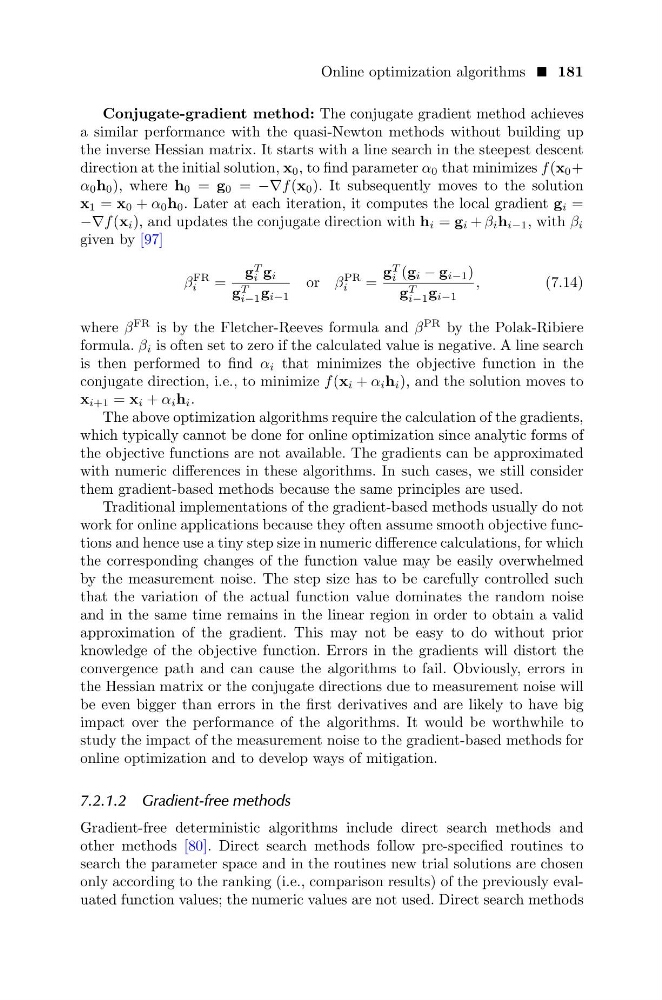
Conjugate-gradient method: The conjugate gradient method achieves
a similar performance with the quasi-Newton methods without building up
the inverse Hessian matrix. It starts with a line search in the steepest descent
direction at the initial solution, x 0 , to find parameter α 0 that minimizes f (x 0 +
α 0 h 0 ), where h 0 = g 0 = −∇f (x 0 ). It subsequently moves to the solution
x 1 = x 0 + α 0 h 0 . Later at each iteration, it computes the local gradient g i =
−∇f (x i ), and updates the conjugate direction with h i = g i + β i h i−1 , with β i
given by [97]
β
FR
i
=
g
T
i g i
g T
i−1 g i−1
or β
PR
i
=
g
T
i (g i − g i−1 )
g T
i−1 g i−1
,
(7.14)
where β
FR is by the Fletcher-Reeves formula and β
PR by the Polak-Ribiere
formula. β i is often set to zero if the calculated value is negative. A line search
is then performed to find α i that minimizes the objective function in the
conjugate direction, i.e., to minimize f (x i + α i h i ), and the solution moves to
x i+1 = x i + α i h i .
The above optimization algorithms require the calculation of the gradients,
which typically cannot be done for online optimization since analytic forms of
the objective functions are not available. The gradients can be approximated
with numeric differences in these algorithms. In such cases, we still consider
them gradient-based methods because the same principles are used.
Traditional implementations of the gradient-based methods usually do not
work for online applications because they often assume smooth objective functions and hence use a tiny step size in numeric difference calculations, for which
the corresponding changes of the function value may be easily overwhelmed
by the measurement noise. The step size has to be carefully controlled such
that the variation of the actual function value dominates the random noise
and in the same time remains in the linear region in order to obtain a valid
approximation of the gradient. This may not be easy to do without prior
knowledge of the objective function. Errors in the gradients will distort the
convergence path and can cause the algorithms to fail. Obviously, errors in
the Hessian matrix or the conjugate directions due to measurement noise will
be even bigger than errors in the first derivatives and are likely to have big
impact over the performance of the algorithms. It would be worthwhile to
study the impact of the measurement noise to the gradient-based methods for
online optimization and to develop ways of mitigation.
7.2.1.2 Gradient-free methods
Gradient-free deterministic algorithms include direct search methods and
other methods [80]. Direct search methods follow pre-specified routines to
search the parameter space and in the routines new trial solutions are chosen
only according to the ranking (i.e., comparison results) of the previously evaluated function values; the numeric values are not used. Direct search methods
Conjugate-gradient method: The conjugate gradient method achieves
a similar performance with the quasi-Newton methods without building up
the inverse Hessian matrix. It starts with a line search in the steepest descent
direction at the initial solution, x 0 , to find parameter α 0 that minimizes f (x 0 +
α 0 h 0 ), where h 0 = g 0 = −∇f (x 0 ). It subsequently moves to the solution
x 1 = x 0 + α 0 h 0 . Later at each iteration, it computes the local gradient g i =
−∇f (x i ), and updates the conjugate direction with h i = g i + β i h i−1 , with β i
given by [97]
β
FR
i
=
g
T
i g i
g T
i−1 g i−1
or β
PR
i
=
g
T
i (g i − g i−1 )
g T
i−1 g i−1
,
(7.14)
where β
FR is by the Fletcher-Reeves formula and β
PR by the Polak-Ribiere
formula. β i is often set to zero if the calculated value is negative. A line search
is then performed to find α i that minimizes the objective function in the
conjugate direction, i.e., to minimize f (x i + α i h i ), and the solution moves to
x i+1 = x i + α i h i .
The above optimization algorithms require the calculation of the gradients,
which typically cannot be done for online optimization since analytic forms of
the objective functions are not available. The gradients can be approximated
with numeric differences in these algorithms. In such cases, we still consider
them gradient-based methods because the same principles are used.
Traditional implementations of the gradient-based methods usually do not
work for online applications because they often assume smooth objective functions and hence use a tiny step size in numeric difference calculations, for which
the corresponding changes of the function value may be easily overwhelmed
by the measurement noise. The step size has to be carefully controlled such
that the variation of the actual function value dominates the random noise
and in the same time remains in the linear region in order to obtain a valid
approximation of the gradient. This may not be easy to do without prior
knowledge of the objective function. Errors in the gradients will distort the
convergence path and can cause the algorithms to fail. Obviously, errors in
the Hessian matrix or the conjugate directions due to measurement noise will
be even bigger than errors in the first derivatives and are likely to have big
impact over the performance of the algorithms. It would be worthwhile to
study the impact of the measurement noise to the gradient-based methods for
online optimization and to develop ways of mitigation.
7.2.1.2 Gradient-free methods
Gradient-free deterministic algorithms include direct search methods and
other methods [80]. Direct search methods follow pre-specified routines to
search the parameter space and in the routines new trial solutions are chosen
only according to the ranking (i.e., comparison results) of the previously evaluated function values; the numeric values are not used. Direct search methods