

172 Beam-based Correction and Optimization for Accelerators
System
f (x)
. . .
x 1
x 2
x n
y 1 = f 1 (x) + ξ 1
y 2 = f 2 (x) + ξ 2
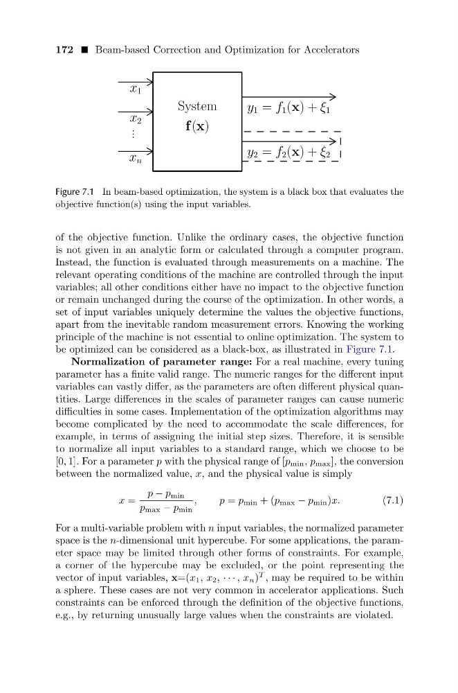
Figure 7.1 In beam-based optimization, the system is a black box that evaluates the
objective function(s) using the input variables.
of the objective function. Unlike the ordinary cases, the objective function
is not given in an analytic form or calculated through a computer program.
Instead, the function is evaluated through measurements on a machine. The
relevant operating conditions of the machine are controlled through the input
variables; all other conditions either have no impact to the objective function
or remain unchanged during the course of the optimization. In other words, a
set of input variables uniquely determine the values the objective functions,
apart from the inevitable random measurement errors. Knowing the working
principle of the machine is not essential to online optimization. The system to
be optimized can be considered as a black-box, as illustrated in Figure 7.1.
Normalization of parameter range: For a real machine, every tuning
parameter has a finite valid range. The numeric ranges for the different input
variables can vastly differ, as the parameters are often different physical quantities. Large differences in the scales of parameter ranges can cause numeric
difficulties in some cases. Implementation of the optimization algorithms may
become complicated by the need to accommodate the scale differences, for
example, in terms of assigning the initial step sizes. Therefore, it is sensible
to normalize all input variables to a standard range, which we choose to be
[0, 1]. For a parameter p with the physical range of [p min , p max ], the conversion
between the normalized value, x, and the physical value is simply
x =
p − p min
p max − p min
,
p = p min + (p max − p min )x.
(7.1)
For a multi-variable problem with n input variables, the normalized parameter
space is the n-dimensional unit hypercube. For some applications, the parameter space may be limited through other forms of constraints. For example,
a corner of the hypercube may be excluded, or the point representing the
vector of input variables, x=(x 1 , x 2 , · · · , x n )
T , may be required to be within
a sphere. These cases are not very common in accelerator applications. Such
constraints can be enforced through the definition of the objective functions,
e.g., by returning unusually large values when the constraints are violated.
System
f (x)
. . .
x 1
x 2
x n
y 1 = f 1 (x) + ξ 1
y 2 = f 2 (x) + ξ 2
Figure 7.1 In beam-based optimization, the system is a black box that evaluates the
objective function(s) using the input variables.
of the objective function. Unlike the ordinary cases, the objective function
is not given in an analytic form or calculated through a computer program.
Instead, the function is evaluated through measurements on a machine. The
relevant operating conditions of the machine are controlled through the input
variables; all other conditions either have no impact to the objective function
or remain unchanged during the course of the optimization. In other words, a
set of input variables uniquely determine the values the objective functions,
apart from the inevitable random measurement errors. Knowing the working
principle of the machine is not essential to online optimization. The system to
be optimized can be considered as a black-box, as illustrated in Figure 7.1.
Normalization of parameter range: For a real machine, every tuning
parameter has a finite valid range. The numeric ranges for the different input
variables can vastly differ, as the parameters are often different physical quantities. Large differences in the scales of parameter ranges can cause numeric
difficulties in some cases. Implementation of the optimization algorithms may
become complicated by the need to accommodate the scale differences, for
example, in terms of assigning the initial step sizes. Therefore, it is sensible
to normalize all input variables to a standard range, which we choose to be
[0, 1]. For a parameter p with the physical range of [p min , p max ], the conversion
between the normalized value, x, and the physical value is simply
x =
p − p min
p max − p min
,
p = p min + (p max − p min )x.
(7.1)
For a multi-variable problem with n input variables, the normalized parameter
space is the n-dimensional unit hypercube. For some applications, the parameter space may be limited through other forms of constraints. For example,
a corner of the hypercube may be excluded, or the point representing the
vector of input variables, x=(x 1 , x 2 , · · · , x n )
T , may be required to be within
a sphere. These cases are not very common in accelerator applications. Such
constraints can be enforced through the definition of the objective functions,
e.g., by returning unusually large values when the constraints are violated.