

156 Beam-based Correction and Optimization for Accelerators
with B and R as defined in Eq. (1.60). The beam motion can then be related
to the normal mode coordinates, Θ, through [83]
X(n) = PΘ(n), with Θ(n) =
√
2J 1 cos Φ 1 (n)
−
√
2J 1 sin Φ 1 (n)
√
2J 2 cos Φ 2 (n)
−
√
2J 2 sin Φ 2 (n)
,
(6.4)
where P ≡ VU, Φ 1,2 (n) = 2πν 1,2 n + φ 1,2 , and J 1,2 and φ 1,2 are action
and angle coordinates for the two normal modes as determined by the initial
conditions. The values of φ 1,2 at different BPMs differ by the phase advances
of the normal modes.
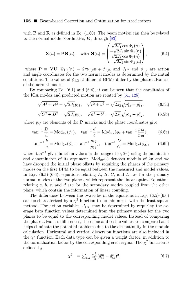
By comparing Eq. (6.1) and (6.4), it can be seen that the amplitudes of
the ICA modes and predicted motion are related by [51, 125]
A 2 + B 2 =
2J 1 p 11 ,
c 2 + d 2 =
2J 2
p 2
13 + p 2
14 ,
(6.5a)
C 2 + D 2 =
2J 2 p 33 ,
a 2 + b 2 =
2J 1
p 2
31 + p 2
32 ,
(6.5b)
where p ij are elements of the P matrix and the phase coordinates give
tan
−1 B
A
= Mod 2π (φ 1 ), tan
−1 d
c
= Mod 2π (φ 2 + tan
−1 p 14
p 13
),
(6.6a)
tan
−1 b
a
= Mod 2π (φ 1 + tan
−1 p 32
p 31
), tan
−1 D
C
= Mod 2π (φ 2 ),
(6.6b)
where tan
−1 gives function values in the range of [0, 2π) using the nominator
and denominator of its argument, Mod 2π (·) denotes modulo of 2π and we
have dropped the initial phase offsets by requiring the phases of the primary
modes on the first BPM to be equal between the measured and model values.
In Eqs. (6.5)-(6.6), equations relating A, B, C, and D are for the primary
normal modes of the two planes, which represent the linear optics. Equations
relating a, b, c, and d are for the secondary modes coupled from the other
plane, which contain the information of linear coupling.
The differences between the two sides in the equations in Eqs. (6.5)-(6.6)
can be characterized by a χ
2 function to be minimized with the least-square
method. The action variables, J 1,2 , may be determined by requiring the average beta function values determined from the primary modes for the two
planes to be equal to the corresponding model values. Instead of comparing
the phase advances differences, their sine and cosine values are compared as it
helps eliminate the potential problems due to the discontinuity in the modulo
calculation. Horizontal and vertical dispersion functions are also included in
the χ
2 function. Each data type can be given a weight factor, in addition to
the normalization factor by the corresponding error sigma. The χ
2 function is
defined by
χ
2 =
i,k
w
2
k
σ 2
ik
(d
m
ik − d
c
ik )
2 ,
(6.7)
with B and R as defined in Eq. (1.60). The beam motion can then be related
to the normal mode coordinates, Θ, through [83]
X(n) = PΘ(n), with Θ(n) =
√
2J 1 cos Φ 1 (n)
−
√
2J 1 sin Φ 1 (n)
√
2J 2 cos Φ 2 (n)
−
√
2J 2 sin Φ 2 (n)
,
(6.4)
where P ≡ VU, Φ 1,2 (n) = 2πν 1,2 n + φ 1,2 , and J 1,2 and φ 1,2 are action
and angle coordinates for the two normal modes as determined by the initial
conditions. The values of φ 1,2 at different BPMs differ by the phase advances
of the normal modes.
By comparing Eq. (6.1) and (6.4), it can be seen that the amplitudes of
the ICA modes and predicted motion are related by [51, 125]
A 2 + B 2 =
2J 1 p 11 ,
c 2 + d 2 =
2J 2
p 2
13 + p 2
14 ,
(6.5a)
C 2 + D 2 =
2J 2 p 33 ,
a 2 + b 2 =
2J 1
p 2
31 + p 2
32 ,
(6.5b)
where p ij are elements of the P matrix and the phase coordinates give
tan
−1 B
A
= Mod 2π (φ 1 ), tan
−1 d
c
= Mod 2π (φ 2 + tan
−1 p 14
p 13
),
(6.6a)
tan
−1 b
a
= Mod 2π (φ 1 + tan
−1 p 32
p 31
), tan
−1 D
C
= Mod 2π (φ 2 ),
(6.6b)
where tan
−1 gives function values in the range of [0, 2π) using the nominator
and denominator of its argument, Mod 2π (·) denotes modulo of 2π and we
have dropped the initial phase offsets by requiring the phases of the primary
modes on the first BPM to be equal between the measured and model values.
In Eqs. (6.5)-(6.6), equations relating A, B, C, and D are for the primary
normal modes of the two planes, which represent the linear optics. Equations
relating a, b, c, and d are for the secondary modes coupled from the other
plane, which contain the information of linear coupling.
The differences between the two sides in the equations in Eqs. (6.5)-(6.6)
can be characterized by a χ
2 function to be minimized with the least-square
method. The action variables, J 1,2 , may be determined by requiring the average beta function values determined from the primary modes for the two
planes to be equal to the corresponding model values. Instead of comparing
the phase advances differences, their sine and cosine values are compared as it
helps eliminate the potential problems due to the discontinuity in the modulo
calculation. Horizontal and vertical dispersion functions are also included in
the χ
2 function. Each data type can be given a weight factor, in addition to
the normalization factor by the corresponding error sigma. The χ
2 function is
defined by
χ
2 =
i,k
w
2
k
σ 2
ik
(d
m
ik − d
c
ik )
2 ,
(6.7)