

Linear optics measurement and correction - II 147
0
1
2
i
beam
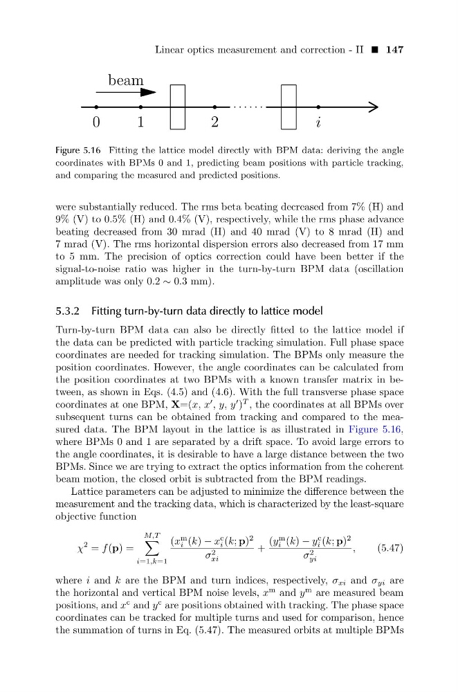
Figure 5.16 Fitting the lattice model directly with BPM data: deriving the angle
coordinates with BPMs 0 and 1, predicting beam positions with particle tracking,
and comparing the measured and predicted positions.
were substantially reduced. The rms beta beating decreased from 7% (H) and
9% (V) to 0.5% (H) and 0.4% (V), respectively, while the rms phase advance
beating decreased from 30 mrad (H) and 40 mrad (V) to 8 mrad (H) and
7 mrad (V). The rms horizontal dispersion errors also decreased from 17 mm
to 5 mm. The precision of optics correction could have been better if the
signal-to-noise ratio was higher in the turn-by-turn BPM data (oscillation
amplitude was only 0.2 ∼ 0.3 mm).
5.3.2 Fitting turn-by-turn data directly to lattice model
Turn-by-turn BPM data can also be directly fitted to the lattice model if
the data can be predicted with particle tracking simulation. Full phase space
coordinates are needed for tracking simulation. The BPMs only measure the
position coordinates. However, the angle coordinates can be calculated from
the position coordinates at two BPMs with a known transfer matrix in between, as shown in Eqs. (4.5) and (4.6). With the full transverse phase space
coordinates at one BPM, X=(x, x
, y, y
)
T , the coordinates at all BPMs over
subsequent turns can be obtained from tracking and compared to the measured data. The BPM layout in the lattice is as illustrated in Figure 5.16,
where BPMs 0 and 1 are separated by a drift space. To avoid large errors to
the angle coordinates, it is desirable to have a large distance between the two
BPMs. Since we are trying to extract the optics information from the coherent
beam motion, the closed orbit is subtracted from the BPM readings.
Lattice parameters can be adjusted to minimize the difference between the
measurement and the tracking data, which is characterized by the least-square
objective function
χ
2 = f (p) =
M,T
i=1,k=1
(x
m
i (k) − x
c
i (k; p)
2
σ 2
xi
+
(y
m
i (k) − y
c
i (k; p)
2
σ 2
yi
,
(5.47)
where i and k are the BPM and turn indices, respectively, σ xi and σ yi are
the horizontal and vertical BPM noise levels, x
m and y
m are measured beam
positions, and x
c and y
c are positions obtained with tracking. The phase space
coordinates can be tracked for multiple turns and used for comparison, hence
the summation of turns in Eq. (5.47). The measured orbits at multiple BPMs
0
1
2
i
beam
Figure 5.16 Fitting the lattice model directly with BPM data: deriving the angle
coordinates with BPMs 0 and 1, predicting beam positions with particle tracking,
and comparing the measured and predicted positions.
were substantially reduced. The rms beta beating decreased from 7% (H) and
9% (V) to 0.5% (H) and 0.4% (V), respectively, while the rms phase advance
beating decreased from 30 mrad (H) and 40 mrad (V) to 8 mrad (H) and
7 mrad (V). The rms horizontal dispersion errors also decreased from 17 mm
to 5 mm. The precision of optics correction could have been better if the
signal-to-noise ratio was higher in the turn-by-turn BPM data (oscillation
amplitude was only 0.2 ∼ 0.3 mm).
5.3.2 Fitting turn-by-turn data directly to lattice model
Turn-by-turn BPM data can also be directly fitted to the lattice model if
the data can be predicted with particle tracking simulation. Full phase space
coordinates are needed for tracking simulation. The BPMs only measure the
position coordinates. However, the angle coordinates can be calculated from
the position coordinates at two BPMs with a known transfer matrix in between, as shown in Eqs. (4.5) and (4.6). With the full transverse phase space
coordinates at one BPM, X=(x, x
, y, y
)
T , the coordinates at all BPMs over
subsequent turns can be obtained from tracking and compared to the measured data. The BPM layout in the lattice is as illustrated in Figure 5.16,
where BPMs 0 and 1 are separated by a drift space. To avoid large errors to
the angle coordinates, it is desirable to have a large distance between the two
BPMs. Since we are trying to extract the optics information from the coherent
beam motion, the closed orbit is subtracted from the BPM readings.
Lattice parameters can be adjusted to minimize the difference between the
measurement and the tracking data, which is characterized by the least-square
objective function
χ
2 = f (p) =
M,T
i=1,k=1
(x
m
i (k) − x
c
i (k; p)
2
σ 2
xi
+
(y
m
i (k) − y
c
i (k; p)
2
σ 2
yi
,
(5.47)
where i and k are the BPM and turn indices, respectively, σ xi and σ yi are
the horizontal and vertical BPM noise levels, x
m and y
m are measured beam
positions, and x
c and y
c are positions obtained with tracking. The phase space
coordinates can be tracked for multiple turns and used for comparison, hence
the summation of turns in Eq. (5.47). The measured orbits at multiple BPMs