

116 Beam-based Correction and Optimization for Accelerators
where the coefficients c i , i = 1, 2, · · · , N q , define the vector c in the
quadrupole parameter space. It is not easy to intuitively come up with underconstrained directions that are more complex than the simple case with adjacent quadrupoles. However, it is straightforward to determine these directions
computationally. In fact, the SV modes of the Jacobian matrix with low singular values are the ultimate representation of the under-constrained directions.
To put on constraints to the SV modes, the χ
2 definition can be modified with
new terms as follows
χ
2
c = χ
2 +
Nq
i=1
w
2
i
σ 2
K
(v
T
K,i ∆K)
2 ,
(4.44)
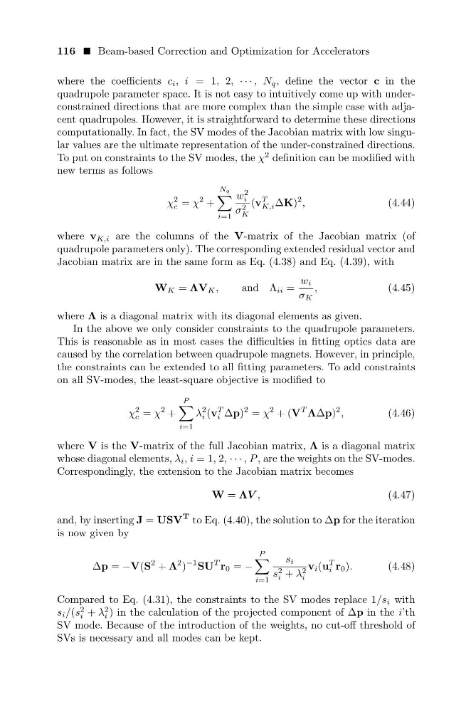
where v K,i are the columns of the V-matrix of the Jacobian matrix (of
quadrupole parameters only). The corresponding extended residual vector and
Jacobian matrix are in the same form as Eq. (4.38) and Eq. (4.39), with
W K = ΛV K ,
and Λ ii =
w i
σ K
,
(4.45)
where Λ is a diagonal matrix with its diagonal elements as given.
In the above we only consider constraints to the quadrupole parameters.
This is reasonable as in most cases the difficulties in fitting optics data are
caused by the correlation between quadrupole magnets. However, in principle,
the constraints can be extended to all fitting parameters. To add constraints
on all SV-modes, the least-square objective is modified to
χ
2
c = χ
2 +
P
i=1
λ
2
i (v
T
i ∆p)
2 = χ
2 + (V
T Λ∆p)
2 ,
(4.46)
where V is the V-matrix of the full Jacobian matrix, Λ is a diagonal matrix
whose diagonal elements, λ i , i = 1, 2, · · · , P , are the weights on the SV-modes.
Correspondingly, the extension to the Jacobian matrix becomes
W = ΛV ,
(4.47)
and, by inserting J = USV
T to Eq. (4.40), the solution to ∆p for the iteration
is now given by
∆p = −V(S
2 + Λ
2 )
−1 SU
T r 0 = −
P
i=1
s i
s 2
i + λ 2
i
v i (u
T
i r 0 ).
(4.48)
Compared to Eq. (4.31), the constraints to the SV modes replace 1/s i with
s i /(s
2
i + λ
2
i ) in the calculation of the projected component of ∆p in the i’th
SV mode. Because of the introduction of the weights, no cut-off threshold of
SVs is necessary and all modes can be kept.
where the coefficients c i , i = 1, 2, · · · , N q , define the vector c in the
quadrupole parameter space. It is not easy to intuitively come up with underconstrained directions that are more complex than the simple case with adjacent quadrupoles. However, it is straightforward to determine these directions
computationally. In fact, the SV modes of the Jacobian matrix with low singular values are the ultimate representation of the under-constrained directions.
To put on constraints to the SV modes, the χ
2 definition can be modified with
new terms as follows
χ
2
c = χ
2 +
Nq
i=1
w
2
i
σ 2
K
(v
T
K,i ∆K)
2 ,
(4.44)
where v K,i are the columns of the V-matrix of the Jacobian matrix (of
quadrupole parameters only). The corresponding extended residual vector and
Jacobian matrix are in the same form as Eq. (4.38) and Eq. (4.39), with
W K = ΛV K ,
and Λ ii =
w i
σ K
,
(4.45)
where Λ is a diagonal matrix with its diagonal elements as given.
In the above we only consider constraints to the quadrupole parameters.
This is reasonable as in most cases the difficulties in fitting optics data are
caused by the correlation between quadrupole magnets. However, in principle,
the constraints can be extended to all fitting parameters. To add constraints
on all SV-modes, the least-square objective is modified to
χ
2
c = χ
2 +
P
i=1
λ
2
i (v
T
i ∆p)
2 = χ
2 + (V
T Λ∆p)
2 ,
(4.46)
where V is the V-matrix of the full Jacobian matrix, Λ is a diagonal matrix
whose diagonal elements, λ i , i = 1, 2, · · · , P , are the weights on the SV-modes.
Correspondingly, the extension to the Jacobian matrix becomes
W = ΛV ,
(4.47)
and, by inserting J = USV
T to Eq. (4.40), the solution to ∆p for the iteration
is now given by
∆p = −V(S
2 + Λ
2 )
−1 SU
T r 0 = −
P
i=1
s i
s 2
i + λ 2
i
v i (u
T
i r 0 ).
(4.48)
Compared to Eq. (4.31), the constraints to the SV modes replace 1/s i with
s i /(s
2
i + λ
2
i ) in the calculation of the projected component of ∆p in the i’th
SV mode. Because of the introduction of the weights, no cut-off threshold of
SVs is necessary and all modes can be kept.