

77
In this paper, we present a detailed methodology to apply PCA, as a simple decorrelation
approach of a compositional dataset, and show its application and performance in a Nickel
laterite deposit.
2 NOTATION
In this paper, the original variable is successively transformed several times, so, we provide
notation to help the reader:
• p – 1 is the dimension of the original vector variable.
• p is the dimension of the vector variable after adding the filler to complete 100%.
• n is the number of data samples.
• X
original is the (p – 1) dimensional vector with the original variable.
• X is the (p) dimensional vector with the original variable, including the filler variable.
• Z is the (p – 1) dimensional vector of additive log-ratios.
• F is the (p – 1) dimensional vector of principal components computed from the log-ratios.
• Y is the (p – 1) dimensional vector of normal scores of the principal components computed
from the log-ratios.
3 METHODOLOGY
The proposed methodology requires three sequential transformations of the data prior to
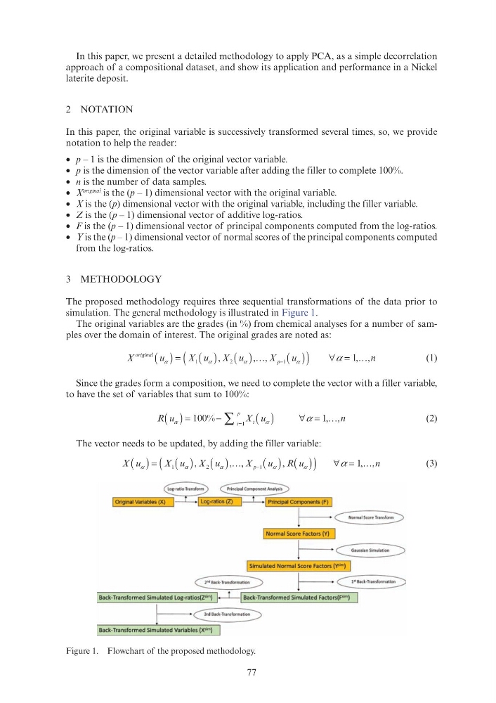
simulation. The general methodology is illustrated in Figure 1.
The original variables are the grades (in %) from chemical analyses for a number of samples over the domain of interest. The original grades are noted as:
X
X
X
X
n
original
p
X
p
( )
u α =
( )
u α
( )
u α
( )
u α
(
) ∀ =
α
…
2
X X
X
X
)
u α
u
1
,
( )
u α
2
X X
,
α
)
u α
u
, X X p
X
) ∀α 1 ,
…
(1)
Since the grades form a composition, we need to complete the vector with a filler variable,
to have the set of variables that sum to 100%:
R
n
i
p
i
i
( )
u α =
( )
α
∀
…
=
∑
100
1
1
%
,
X X
p X i
X
i
α
−
( )
u α
u
∀ =
α
∑
1 ,
(2)
The vector needs to be updated, by adding the filler variable:
X
X
X
X
R
n
p
X
p
α
( )
u α =
( )
u α
( )
u α …
( )
α
( )
u
( )
u α
(
) ∀ =
α
2
X X
X
X
)
u α
u
1
,
( )
u α
2
X X
,
)
u α
u
, X X p
X
, ,
…
(3)
Figure 1. Flowchart of the proposed methodology.
I Original Variables (X)
~~
I Normal Score Factors (Y) I
t----~
I Simulated Normal Score Factors (lfim) I
In this paper, we present a detailed methodology to apply PCA, as a simple decorrelation
approach of a compositional dataset, and show its application and performance in a Nickel
laterite deposit.
2 NOTATION
In this paper, the original variable is successively transformed several times, so, we provide
notation to help the reader:
• p – 1 is the dimension of the original vector variable.
• p is the dimension of the vector variable after adding the filler to complete 100%.
• n is the number of data samples.
• X
original is the (p – 1) dimensional vector with the original variable.
• X is the (p) dimensional vector with the original variable, including the filler variable.
• Z is the (p – 1) dimensional vector of additive log-ratios.
• F is the (p – 1) dimensional vector of principal components computed from the log-ratios.
• Y is the (p – 1) dimensional vector of normal scores of the principal components computed
from the log-ratios.
3 METHODOLOGY
The proposed methodology requires three sequential transformations of the data prior to
simulation. The general methodology is illustrated in Figure 1.
The original variables are the grades (in %) from chemical analyses for a number of samples over the domain of interest. The original grades are noted as:
X
X
X
X
n
original
p
X
p
( )
u α =
( )
u α
( )
u α
( )
u α
(
) ∀ =
α
…
2
X X
X
X
)
u α
u
1
,
( )
u α
2
X X
,
α
)
u α
u
, X X p
X
) ∀α 1 ,
…
(1)
Since the grades form a composition, we need to complete the vector with a filler variable,
to have the set of variables that sum to 100%:
R
n
i
p
i
i
( )
u α =
( )
α
∀
…
=
∑
100
1
1
%
,
X X
p X i
X
i
α
−
( )
u α
u
∀ =
α
∑
1 ,
(2)
The vector needs to be updated, by adding the filler variable:
X
X
X
X
R
n
p
X
p
α
( )
u α =
( )
u α
( )
u α …
( )
α
( )
u
( )
u α
(
) ∀ =
α
2
X X
X
X
)
u α
u
1
,
( )
u α
2
X X
,
)
u α
u
, X X p
X
, ,
…
(3)
Figure 1. Flowchart of the proposed methodology.
I Original Variables (X)
~~
I Normal Score Factors (Y) I
t----~
I Simulated Normal Score Factors (lfim) I