

68
The LVA field specifies the local orientation and aspect ratio of the anisotropy field at each
grid cell (block center) location, which varies throughout the model space. Copper, gold and
silver at Grasberg have circular continuity in plan view but near vertical continuity in cross
section, so the local anisotropy is defined by a horizontal direction (rotation about z-axis) and
aspect ratios of the horizontal (major: semi-major) and vertical (major: vertical) anisotropy.
Rather than using the Euclidean or linear straight line distance between points to calculate
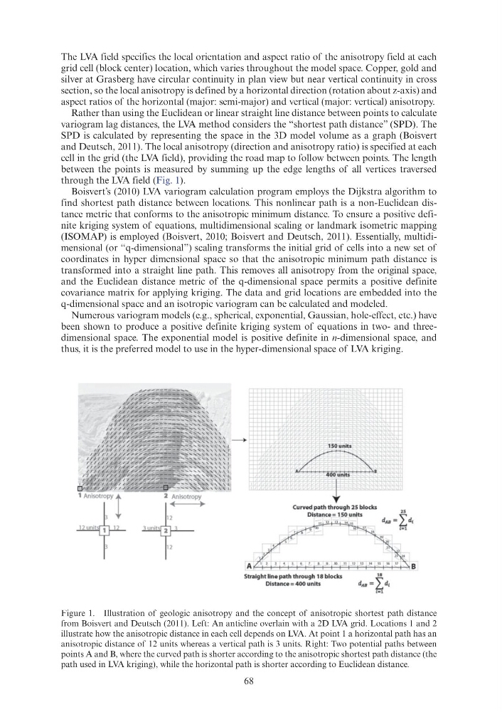
variogram lag distances, the LVA method considers the “shortest path distance” (SPD). The
SPD is calculated by representing the space in the 3D model volume as a graph (Boisvert
and Deutsch, 2011). The local anisotropy (direction and anisotropy ratio) is specified at each
cell in the grid (the LVA field), providing the road map to follow between points. The length
between the points is measured by summing up the edge lengths of all vertices traversed
through the LVA field (Fig. 1).
Boisvert’s (2010) LVA variogram calculation program employs the Dijkstra algorithm to
find shortest path distance between locations. This nonlinear path is a non-Euclidean distance metric that conforms to the anisotropic minimum distance. To ensure a positive definite kriging system of equations, multidimensional scaling or landmark isometric mapping
(ISOMAP) is employed (Boisvert, 2010; Boisvert and Deutsch, 2011). Essentially, multidimensional (or “q-dimensional”) scaling transforms the initial grid of cells into a new set of
coordinates in hyper dimensional space so that the anisotropic minimum path distance is
transformed into a straight line path. This removes all anisotropy from the original space,
and the Euclidean distance metric of the q-dimensional space permits a positive definite
covariance matrix for applying kriging. The data and grid locations are embedded into the
q-dimensional space and an isotropic variogram can be calculated and modeled.
Numerous variogram models (e.g., spherical, exponential, Gaussian, hole-effect, etc.) have
been shown to produce a positive definite kriging system of equations in two- and threedimensional space. The exponential model is positive definite in n-dimensional space, and
thus, it is the preferred model to use in the hyper-dimensional space of LVA kriging.
Figure 1. Illustration of geologic anisotropy and the concept of anisotropic shortest path distance
from Boisvert and Deutsch (2011). Left: An anticline overlain with a 2D LVA grid. Locations 1 and 2
illustrate how the anisotropic distance in each cell depends on LVA. At point 1 a horizontal path has an
anisotropic distance of 12 units whereas a vertical path is 3 units. Right: Two potential paths between
points A and B, where the curved path is shorter according to the anisotropic shortest path distance (the
path used in LVA kriging), while the horizontal path is shorter according to Euclidean distance.
; -
~: lit: "_: '
r
\1
\ I
\ I<
\ I
\ I
\ I
~ :
\ I
Curved path through 25 blocks
Distance= 150 units
Straight line path through 18 blocks
Distance= 400 unit s
18
dA• =Ld,
1•1
The LVA field specifies the local orientation and aspect ratio of the anisotropy field at each
grid cell (block center) location, which varies throughout the model space. Copper, gold and
silver at Grasberg have circular continuity in plan view but near vertical continuity in cross
section, so the local anisotropy is defined by a horizontal direction (rotation about z-axis) and
aspect ratios of the horizontal (major: semi-major) and vertical (major: vertical) anisotropy.
Rather than using the Euclidean or linear straight line distance between points to calculate
variogram lag distances, the LVA method considers the “shortest path distance” (SPD). The
SPD is calculated by representing the space in the 3D model volume as a graph (Boisvert
and Deutsch, 2011). The local anisotropy (direction and anisotropy ratio) is specified at each
cell in the grid (the LVA field), providing the road map to follow between points. The length
between the points is measured by summing up the edge lengths of all vertices traversed
through the LVA field (Fig. 1).
Boisvert’s (2010) LVA variogram calculation program employs the Dijkstra algorithm to
find shortest path distance between locations. This nonlinear path is a non-Euclidean distance metric that conforms to the anisotropic minimum distance. To ensure a positive definite kriging system of equations, multidimensional scaling or landmark isometric mapping
(ISOMAP) is employed (Boisvert, 2010; Boisvert and Deutsch, 2011). Essentially, multidimensional (or “q-dimensional”) scaling transforms the initial grid of cells into a new set of
coordinates in hyper dimensional space so that the anisotropic minimum path distance is
transformed into a straight line path. This removes all anisotropy from the original space,
and the Euclidean distance metric of the q-dimensional space permits a positive definite
covariance matrix for applying kriging. The data and grid locations are embedded into the
q-dimensional space and an isotropic variogram can be calculated and modeled.
Numerous variogram models (e.g., spherical, exponential, Gaussian, hole-effect, etc.) have
been shown to produce a positive definite kriging system of equations in two- and threedimensional space. The exponential model is positive definite in n-dimensional space, and
thus, it is the preferred model to use in the hyper-dimensional space of LVA kriging.
Figure 1. Illustration of geologic anisotropy and the concept of anisotropic shortest path distance
from Boisvert and Deutsch (2011). Left: An anticline overlain with a 2D LVA grid. Locations 1 and 2
illustrate how the anisotropic distance in each cell depends on LVA. At point 1 a horizontal path has an
anisotropic distance of 12 units whereas a vertical path is 3 units. Right: Two potential paths between
points A and B, where the curved path is shorter according to the anisotropic shortest path distance (the
path used in LVA kriging), while the horizontal path is shorter according to Euclidean distance.
; -
~: lit: "_: '
r
\1
\ I
\ I<
\ I
\ I
\ I
~ :
\ I
Curved path through 25 blocks
Distance= 150 units
Straight line path through 18 blocks
Distance= 400 unit s
18
dA• =Ld,
1•1