

528
beginning of the shift, the machine is going to the mining face, after loading by LHD, the
HT goes to unloading point, release ore and goes back to mining face. The whole process may take (depending on distance) c.a. from several to dozen minutes. Due to a number
of machines operating in given mining departments and other factors related to “normal”
operation of the underground mine, the transportation process might be disturbed for each
cycle (HT must stop for a while because the loading process appeared more complicated, or
unloading process is blocked due to oversized ore pieces etc.). Such disturbances mean that
cycles may have some variation in time and it brings extra complexity during analysis. Anyway, the cyclic nature of the process is the basis for further analysis in this paper.
3.2 Autocorrelation function
Autocorrelation function (ACF) describes the correlation of a signal with a delayed copy of
itself as a function of delay. In other words, it measures the similarity between observations as
a function of the time lag between them. The analysis of autocorrelation might be considered
as a mathematical tool for finding repeating patterns (i.e. operational cycle for haulage).
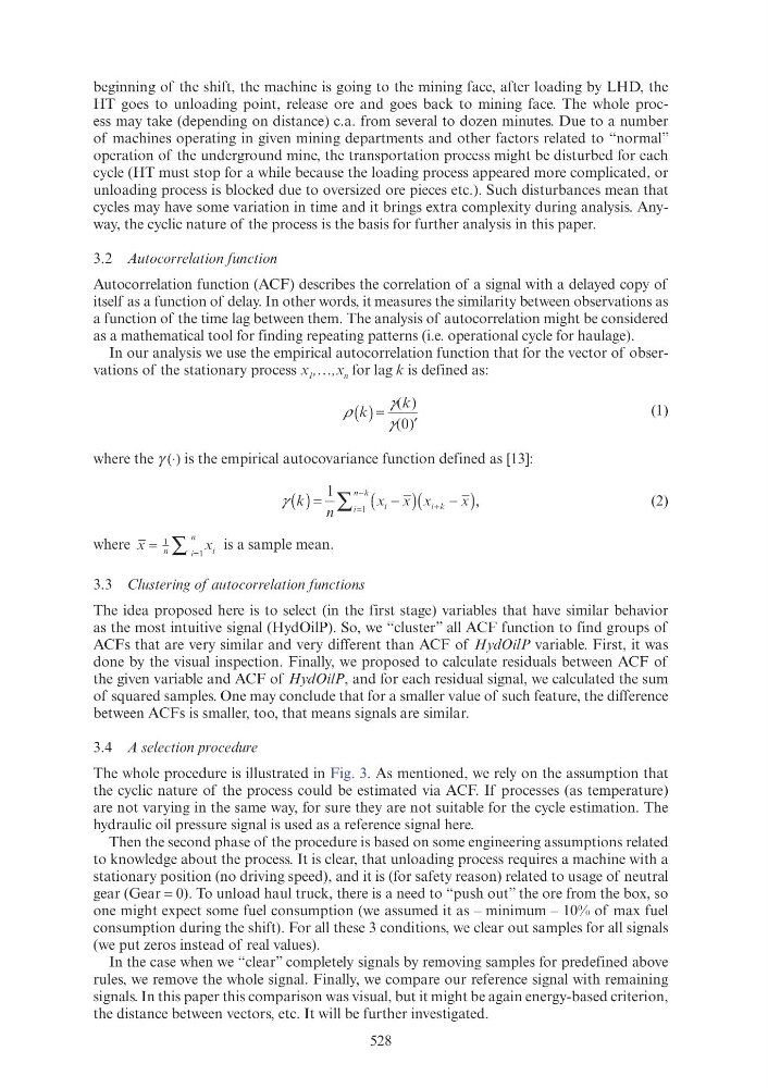
In our analysis we use the empirical autocorrelation function that for the vector of observations of the stationary process x 1 ,…,x n for lag k is defined as:
ρ
γ
γ
( )
k =
′
( )
γ γ k
( )
γ γ
(1)
where the γ (⋅) is the empirical autocovariance function defined as [13]:
γ
n
i
n k
( )
k =
(
)
x x
i
x
(
)
x
x
i k
=
∑
1
1
,
(2)
where x
x
n
i
i
n
=
∑
1
1
is a sample mean.
3.3 Clustering of autocorrelation functions
The idea proposed here is to select (in the first stage) variables that have similar behavior
as the most intuitive signal (HydOilP). So, we “cluster” all ACF function to find groups of
ACFs that are very similar and very different than ACF of HydOilP variable. First, it was
done by the visual inspection. Finally, we proposed to calculate residuals between ACF of
the given variable and ACF of HydOilP, and for each residual signal, we calculated the sum
of squared samples. One may conclude that for a smaller value of such feature, the difference
between ACFs is smaller, too, that means signals are similar.
3.4 A selection procedure
The whole procedure is illustrated in Fig. 3. As mentioned, we rely on the assumption that
the cyclic nature of the process could be estimated via ACF. If processes (as temperature)
are not varying in the same way, for sure they are not suitable for the cycle estimation. The
hydraulic oil pressure signal is used as a reference signal here.
Then the second phase of the procedure is based on some engineering assumptions related
to knowledge about the process. It is clear, that unloading process requires a machine with a
stationary position (no driving speed), and it is (for safety reason) related to usage of neutral
gear (Gear = 0). To unload haul truck, there is a need to “push out” the ore from the box, so
one might expect some fuel consumption (we assumed it as – minimum – 10% of max fuel
consumption during the shift). For all these 3 conditions, we clear out samples for all signals
(we put zeros instead of real values).
In the case when we “clear” completely signals by removing samples for predefined above
rules, we remove the whole signal. Finally, we compare our reference signal with remaining
signals. In this paper this comparison was visual, but it might be again energy-based criterion,
the distance between vectors, etc. It will be further investigated.