

415
Researchers at Adolfo Ibañez University and University of Chile, Santiago, have developed a
tool, OMP Solver that leverages these new algorithms to solve both surface and underground
scheduling problems. The following section presents a special feature that can be used with
OMP Solver to create models with greater tractability and in producing more operationally
representative schedules.
2.1.1 Multi-Time period knapsack constraints
Mining operations often use production averages to create strategic and tactical schedules.
These averages might reflect the daily, weekly or even monthly production rates for a given
mining method or activity, often corresponding to the fidelity of the desired schedule. Considering the highly variable activity durations typically seen at underground mining operations,
because of the non-homogeneous nature of the mine design, using averages may leave available production unscheduled. For example, the assigned production rate for stope extraction
is 500 tons per day; however, the average mine production requirement over the year may be
1200 tons per day. When using an integer program, this means that the production capacity will be under-utilized by 200 tons per day, assuming that two stopes are available to be
scheduled each day. Many practitioners have incorporated continuous variables (Nehring
and Topal, 2007; Little et al., 2008), in conjunction with integer variables, to account for
this occurrence; yet, there are still challenges associated with solving such large-scale mixed
integer problems.
To retain an integer formulation, an alternative was developed that provides the flexibility
similar to that seen in mixed integer programs while allowing the use of newer solution methods. We present Multi-time Period Knapsack Constraints (MPKC) that allow practitioners to create schedules with variable production volumes, by achieving a production target
or limiting resource capacities measured over multiple time periods. For example, a mine’s
production output can vary from day-to-day, but the ore production target is set annually.
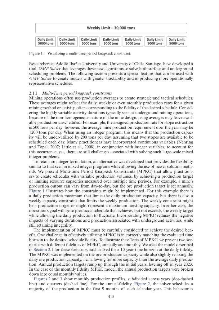
Figure 1 illustrates how the constraints might be implemented. For this example there is
a daily production maximum that limits the daily production capacity, but there is also a
weekly capacity constraint that limits the weekly production. The weekly constraint might
be a production target or might represent a maximum hoisting capacity. In either case, the
operation’s goal will be to produce a schedule that achieves, but not exceeds, the weekly target
while allowing the daily production to fluctuate. Incorporating MPKC reduces the negative
impacts of varying durations and production associated with underground activities, while
still retaining integrality.
The implementation of MPKC must be carefully considered to achieve the desired benefit. One challenge in effectively utilizing MPKC is in correctly matching the evaluated time
horizon to the desired schedule fidelity. To illustrate the effects of MPKC, we present two scenarios with different fidelities of MPKC, annually and monthly. We used the model described
in Section 2.1 for these scenarios, each solved for a 10-year time horizon at the daily fidelity.
The MPKC was implemented on the ore production capacity while also slightly relaxing the
daily ore production capacity, i.e., allowing for more capacity than the average daily production. Annual production targets ramp up through the initial years, leveling off in year 2023.
In the case of the monthly fidelity MPKC model, the annual production targets were broken
down into equal monthly values.
Figures 2 and 3 show monthly production profiles, subdivided across years (dot-dashed
line) and quarters (dashed line). For the annual-fidelity, Figure 2, the solver schedules a
majority of the production in the first 9 months of each calendar year. This behavior is
Figure 1. Visualizing a multi-time period knapsack constraint.
Weekly Limit- 30,000 tons
Researchers at Adolfo Ibañez University and University of Chile, Santiago, have developed a
tool, OMP Solver that leverages these new algorithms to solve both surface and underground
scheduling problems. The following section presents a special feature that can be used with
OMP Solver to create models with greater tractability and in producing more operationally
representative schedules.
2.1.1 Multi-Time period knapsack constraints
Mining operations often use production averages to create strategic and tactical schedules.
These averages might reflect the daily, weekly or even monthly production rates for a given
mining method or activity, often corresponding to the fidelity of the desired schedule. Considering the highly variable activity durations typically seen at underground mining operations,
because of the non-homogeneous nature of the mine design, using averages may leave available production unscheduled. For example, the assigned production rate for stope extraction
is 500 tons per day; however, the average mine production requirement over the year may be
1200 tons per day. When using an integer program, this means that the production capacity will be under-utilized by 200 tons per day, assuming that two stopes are available to be
scheduled each day. Many practitioners have incorporated continuous variables (Nehring
and Topal, 2007; Little et al., 2008), in conjunction with integer variables, to account for
this occurrence; yet, there are still challenges associated with solving such large-scale mixed
integer problems.
To retain an integer formulation, an alternative was developed that provides the flexibility
similar to that seen in mixed integer programs while allowing the use of newer solution methods. We present Multi-time Period Knapsack Constraints (MPKC) that allow practitioners to create schedules with variable production volumes, by achieving a production target
or limiting resource capacities measured over multiple time periods. For example, a mine’s
production output can vary from day-to-day, but the ore production target is set annually.
Figure 1 illustrates how the constraints might be implemented. For this example there is
a daily production maximum that limits the daily production capacity, but there is also a
weekly capacity constraint that limits the weekly production. The weekly constraint might
be a production target or might represent a maximum hoisting capacity. In either case, the
operation’s goal will be to produce a schedule that achieves, but not exceeds, the weekly target
while allowing the daily production to fluctuate. Incorporating MPKC reduces the negative
impacts of varying durations and production associated with underground activities, while
still retaining integrality.
The implementation of MPKC must be carefully considered to achieve the desired benefit. One challenge in effectively utilizing MPKC is in correctly matching the evaluated time
horizon to the desired schedule fidelity. To illustrate the effects of MPKC, we present two scenarios with different fidelities of MPKC, annually and monthly. We used the model described
in Section 2.1 for these scenarios, each solved for a 10-year time horizon at the daily fidelity.
The MPKC was implemented on the ore production capacity while also slightly relaxing the
daily ore production capacity, i.e., allowing for more capacity than the average daily production. Annual production targets ramp up through the initial years, leveling off in year 2023.
In the case of the monthly fidelity MPKC model, the annual production targets were broken
down into equal monthly values.
Figures 2 and 3 show monthly production profiles, subdivided across years (dot-dashed
line) and quarters (dashed line). For the annual-fidelity, Figure 2, the solver schedules a
majority of the production in the first 9 months of each calendar year. This behavior is
Figure 1. Visualizing a multi-time period knapsack constraint.
Weekly Limit- 30,000 tons