

334
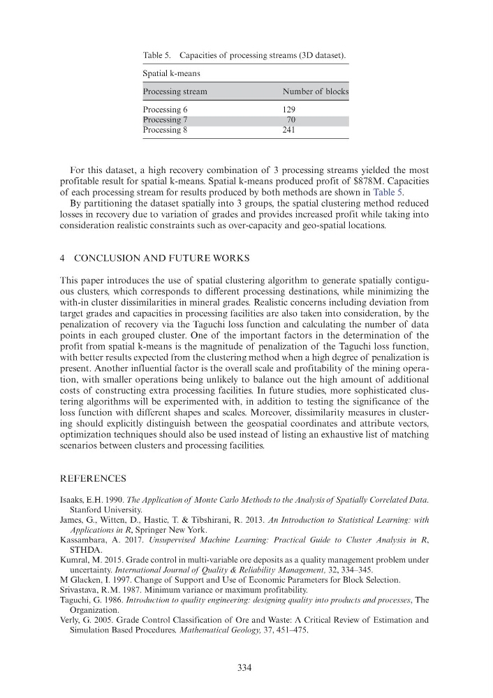
Table 5. Capacities of processing streams (3D dataset).
Spatial k-means
Processing stream
Number of blocks
Processing 6
129
Processing 7
70
Processing 8
241
For this dataset, a high recovery combination of 3 processing streams yielded the most
profitable result for spatial k-means. Spatial k-means produced profit of $878M. Capacities
of each processing stream for results produced by both methods are shown in Table 5.
By partitioning the dataset spatially into 3 groups, the spatial clustering method reduced
losses in recovery due to variation of grades and provides increased profit while taking into
consideration realistic constraints such as over-capacity and geo-spatial locations.
4 CONCLUSION AND FUTURE WORKS
This paper introduces the use of spatial clustering algorithm to generate spatially contiguous clusters, which corresponds to different processing destinations, while minimizing the
with-in cluster dissimilarities in mineral grades. Realistic concerns including deviation from
target grades and capacities in processing facilities are also taken into consideration, by the
penalization of recovery via the Taguchi loss function and calculating the number of data
points in each grouped cluster. One of the important factors in the determination of the
profit from spatial k-means is the magnitude of penalization of the Taguchi loss function,
with better results expected from the clustering method when a high degree of penalization is
present. Another influential factor is the overall scale and profitability of the mining operation, with smaller operations being unlikely to balance out the high amount of additional
costs of constructing extra processing facilities. In future studies, more sophisticated clustering algorithms will be experimented with, in addition to testing the significance of the
loss function with different shapes and scales. Moreover, dissimilarity measures in clustering should explicitly distinguish between the geospatial coordinates and attribute vectors,
optimization techniques should also be used instead of listing an exhaustive list of matching
scenarios between clusters and processing facilities.
REFERENCES
Isaaks, E.H. 1990. The Application of Monte Carlo Methods to the Analysis of Spatially Correlated Data.
Stanford University.
James, G., Witten, D., Hastie, T. & Tibshirani, R. 2013. An Introduction to Statistical Learning: with
Applications in R, Springer New York.
Kassambara, A. 2017. Unsupervised Machine Learning: Practical Guide to Cluster Analysis in R,
STHDA.
Kumral, M. 2015. Grade control in multi-variable ore deposits as a quality management problem under
uncertainty. International Journal of Quality & Reliability Management, 32, 334–345.
M Glacken, I. 1997. Change of Support and Use of Economic Parameters for Block Selection.
Srivastava, R.M. 1987. Minimum variance or maximum profitability.
Taguchi, G. 1986. Introduction to quality engineering: designing quality into products and processes, The
Organization.
Verly, G. 2005. Grade Control Classification of Ore and Waste: A Critical Review of Estimation and
Simulation Based Procedures. Mathematical Geology, 37, 451–475.
Table 5. Capacities of processing streams (3D dataset).
Spatial k-means
Processing stream
Number of blocks
Processing 6
129
Processing 7
70
Processing 8
241
For this dataset, a high recovery combination of 3 processing streams yielded the most
profitable result for spatial k-means. Spatial k-means produced profit of $878M. Capacities
of each processing stream for results produced by both methods are shown in Table 5.
By partitioning the dataset spatially into 3 groups, the spatial clustering method reduced
losses in recovery due to variation of grades and provides increased profit while taking into
consideration realistic constraints such as over-capacity and geo-spatial locations.
4 CONCLUSION AND FUTURE WORKS
This paper introduces the use of spatial clustering algorithm to generate spatially contiguous clusters, which corresponds to different processing destinations, while minimizing the
with-in cluster dissimilarities in mineral grades. Realistic concerns including deviation from
target grades and capacities in processing facilities are also taken into consideration, by the
penalization of recovery via the Taguchi loss function and calculating the number of data
points in each grouped cluster. One of the important factors in the determination of the
profit from spatial k-means is the magnitude of penalization of the Taguchi loss function,
with better results expected from the clustering method when a high degree of penalization is
present. Another influential factor is the overall scale and profitability of the mining operation, with smaller operations being unlikely to balance out the high amount of additional
costs of constructing extra processing facilities. In future studies, more sophisticated clustering algorithms will be experimented with, in addition to testing the significance of the
loss function with different shapes and scales. Moreover, dissimilarity measures in clustering should explicitly distinguish between the geospatial coordinates and attribute vectors,
optimization techniques should also be used instead of listing an exhaustive list of matching
scenarios between clusters and processing facilities.
REFERENCES
Isaaks, E.H. 1990. The Application of Monte Carlo Methods to the Analysis of Spatially Correlated Data.
Stanford University.
James, G., Witten, D., Hastie, T. & Tibshirani, R. 2013. An Introduction to Statistical Learning: with
Applications in R, Springer New York.
Kassambara, A. 2017. Unsupervised Machine Learning: Practical Guide to Cluster Analysis in R,
STHDA.
Kumral, M. 2015. Grade control in multi-variable ore deposits as a quality management problem under
uncertainty. International Journal of Quality & Reliability Management, 32, 334–345.
M Glacken, I. 1997. Change of Support and Use of Economic Parameters for Block Selection.
Srivastava, R.M. 1987. Minimum variance or maximum profitability.
Taguchi, G. 1986. Introduction to quality engineering: designing quality into products and processes, The
Organization.
Verly, G. 2005. Grade Control Classification of Ore and Waste: A Critical Review of Estimation and
Simulation Based Procedures. Mathematical Geology, 37, 451–475.