

329
of the geo-spatial coordinates in the clustering algorithm effectively takes into consideration
orebody accessibility and facilities planning of production rates, so that better balances could
be achieved between production rates and processing capacities.
2 METHODOLOGY
2.1 K-means clustering algorithm with spatial coordinates as additional variables
The clustering technique used in this paper is the k-means clustering with spatial coordinates
as additional variables. i.e. each data point can be written as x i
T
T T
[
]
a s
T
a
T
where
p
R
εR R
a
is the
vector of p attributes of interest and
d
R
εR R
s
represents the vector of geospatial coordinates.
The k-means algorithm partitions a given dataset into k prespecified number of clusters in
such a way that minimizes the with-in cluster dissimilarity and maximizes the inter-cluster
dissimilarity. Various distance measures exist for defining dissimilarity among data points,
including the Euclidean distance, the Manhattan distance and many other correlation-based
distances. Euclidean distance is chosen in this case as it considers exactly the spatial distance
between points. A brief summary of the k-means algorithm is as follows (Kassambara, 2017):
• Randomly select k points as initial cluster centers, with k being a prespecified number
Until convergence or a maximum number of iterations is reached, repeat the follows:
• Assign each data point to a cluster based on the dissimilarity measure between itself and
the cluster centers
• For the k clusters formed, update the cluster centers by taking the average values of all
points in each cluster
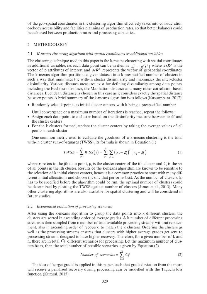
One common metric used to evaluate the goodness of a k-means clustering is the total
with-in cluster sum-of-squares (TWSS), its formula is shown in Equation (1)
TWSS
x j
i
T
j
i
=
(
) (
)
−
=
∑
∑
SS( )
i
i
k
j C
∈
i
k
i
C C
1
1
i
μ μ
μ
x
i i
j
) ( −
x
) (
μ μ i i i i
μ i i
μ μ i i i i
(1)
where x j refers to the jth data point, μ i is the cluster center of the ith cluster and C i is the set
of all points in the ith cluster. Results of the k-means algorithm are known to be sensitive to
the selection of k initial cluster centers, hence it is a common practice to start with many different initial allocations and choose the one that performs best. As the number of clusters, k,
has to be specified before the algorithm could be run, the optimal number of clusters could
be determined by plotting the TWSS against number of clusters (James et al., 2013). Many
other clustering algorithms are also available for spatial clustering and will be considered in
future studies.
2.2 Economical evaluation of processing scenarios
After using the k-means algorithm to group the data points into k different clusters, the
clusters are sorted in ascending order of average grades. A k number of different processing
streams is then sampled from n number of total available processing streams without replacement, also in ascending order of recovery, to match the k clusters. Ordering the clusters as
well as the processing streams ensures that clusters with higher average grades get sent to
processing streams designed to have higher recovery. Therefore, for a given number of k and
n, there are in total C k
C
n different scenarios for processing. Let the maximum number of clusters be m, then the total number of possible scenarios is given by Equation (2).
Number of scenarios
C
k
m
k
C
n
=
∑
1
(2)
The idea of ‘target grade’ is applied in this paper, such that grade deviation from the mean
will receive a penalized recovery during processing can be modelled with the Taguchi loss
function (Kumral, 2015).
of the geo-spatial coordinates in the clustering algorithm effectively takes into consideration
orebody accessibility and facilities planning of production rates, so that better balances could
be achieved between production rates and processing capacities.
2 METHODOLOGY
2.1 K-means clustering algorithm with spatial coordinates as additional variables
The clustering technique used in this paper is the k-means clustering with spatial coordinates
as additional variables. i.e. each data point can be written as x i
T
T T
[
]
a s
T
a
T
where
p
R
εR R
a
is the
vector of p attributes of interest and
d
R
εR R
s
represents the vector of geospatial coordinates.
The k-means algorithm partitions a given dataset into k prespecified number of clusters in
such a way that minimizes the with-in cluster dissimilarity and maximizes the inter-cluster
dissimilarity. Various distance measures exist for defining dissimilarity among data points,
including the Euclidean distance, the Manhattan distance and many other correlation-based
distances. Euclidean distance is chosen in this case as it considers exactly the spatial distance
between points. A brief summary of the k-means algorithm is as follows (Kassambara, 2017):
• Randomly select k points as initial cluster centers, with k being a prespecified number
Until convergence or a maximum number of iterations is reached, repeat the follows:
• Assign each data point to a cluster based on the dissimilarity measure between itself and
the cluster centers
• For the k clusters formed, update the cluster centers by taking the average values of all
points in each cluster
One common metric used to evaluate the goodness of a k-means clustering is the total
with-in cluster sum-of-squares (TWSS), its formula is shown in Equation (1)
TWSS
x j
i
T
j
i
=
(
) (
)
−
=
∑
∑
SS( )
i
i
k
j C
∈
i
k
i
C C
1
1
i
μ μ
μ
x
i i
j
) ( −
x
) (
μ μ i i i i
μ i i
μ μ i i i i
(1)
where x j refers to the jth data point, μ i is the cluster center of the ith cluster and C i is the set
of all points in the ith cluster. Results of the k-means algorithm are known to be sensitive to
the selection of k initial cluster centers, hence it is a common practice to start with many different initial allocations and choose the one that performs best. As the number of clusters, k,
has to be specified before the algorithm could be run, the optimal number of clusters could
be determined by plotting the TWSS against number of clusters (James et al., 2013). Many
other clustering algorithms are also available for spatial clustering and will be considered in
future studies.
2.2 Economical evaluation of processing scenarios
After using the k-means algorithm to group the data points into k different clusters, the
clusters are sorted in ascending order of average grades. A k number of different processing
streams is then sampled from n number of total available processing streams without replacement, also in ascending order of recovery, to match the k clusters. Ordering the clusters as
well as the processing streams ensures that clusters with higher average grades get sent to
processing streams designed to have higher recovery. Therefore, for a given number of k and
n, there are in total C k
C
n different scenarios for processing. Let the maximum number of clusters be m, then the total number of possible scenarios is given by Equation (2).
Number of scenarios
C
k
m
k
C
n
=
∑
1
(2)
The idea of ‘target grade’ is applied in this paper, such that grade deviation from the mean
will receive a penalized recovery during processing can be modelled with the Taguchi loss
function (Kumral, 2015).