

248
tistical distribution of the data and produce biased estimates. “Declustering” can mathematically compensate for this uneven sample spacing and statistical effects caused by correlated
samples.
The GSLib method of declustering calculates weights against a grid overlain on the sample space. This grid goes through a variety of cell sizes to simulate grouping the data into
progressively larger cells. At each size, the grid is slid through a pattern of offsets to limit the
possibility of a calculation through a chance of the grid position. A condition of the declustering calculation is that the sum of the weights must equal the total number of samples,
meaning that individual weights will be either less than or greater than unity.
The objective of the technique is to find the sample spacing that results in the minimum average grade of samples falling within each grid cell which cell, which is by convention a square
rectangle defined by the length of one side. In practice, the weighted average grade will decrease
until it reaches a plateau. Beyond this point, there is no significant change in the declustered
average grade. Beyond a certain cell size and, the declustered mean stabilizes. The resultant
declustering weights are thus inversely proportional to the average spacing between samples.
Two hypothetical case studies described later in this paper are used to help illustrate how
to apply the technique. The first study represents a gold resource for the Middle of Nowhere
gold deposit. The second case study is the Hill Top Iron Ore deposit project in part of a massive magnetite project.
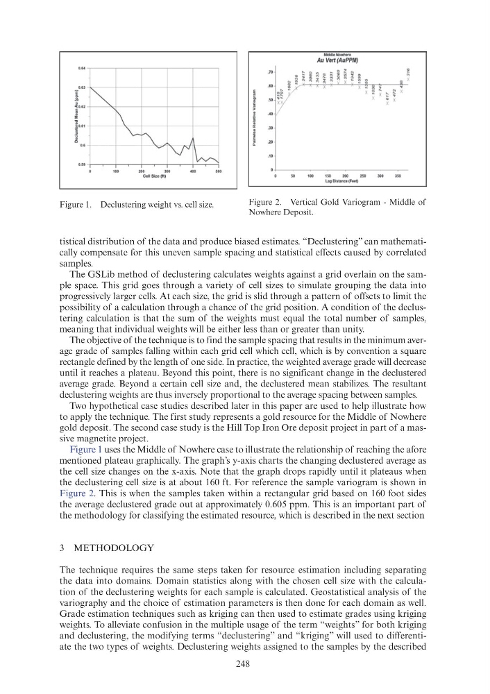
Figure 1 uses the Middle of Nowhere case to illustrate the relationship of reaching the afore
mentioned plateau graphically. The graph’s y-axis charts the changing declustered average as
the cell size changes on the x-axis. Note that the graph drops rapidly until it plateaus when
the declustering cell size is at about 160 ft. For reference the sample variogram is shown in
Figure 2. This is when the samples taken within a rectangular grid based on 160 foot sides
the average declustered grade out at approximately 0.605 ppm. This is an important part of
the methodology for classifying the estimated resource, which is described in the next section
3 METHODOLOGY
The technique requires the same steps taken for resource estimation including separating
the data into domains. Domain statistics along with the chosen cell size with the calculation of the declustering weights for each sample is calculated. Geostatistical analysis of the
variography and the choice of estimation parameters is then done for each domain as well.
Grade estimation techniques such as kriging can then used to estimate grades using kriging
weights. To alleviate confusion in the multiple usage of the term “weights” for both kriging
and declustering, the modifying terms “declustering” and “kriging” will used to differentiate the two types of weights. Declustering weights assigned to the samples by the described
Figure 1. Declustering weight vs. cell size.
Figure 2. Vertical Gold Variogram - Middle of
Nowhere Deposit.
~
g
~
8
~
g
~
Declustered Mean Au (ppm)
; ~
e ::
8 --l- -(.----+--\----t--1
g
Pai rwise Relattve Varlog ram
~
~
~
~
~
~
~~ 4 18
~1 '\ 7~:G82
1936
2 4 17
""
"
~
;,.
1>< 3 060
');;
~
~
x: 103G
tistical distribution of the data and produce biased estimates. “Declustering” can mathematically compensate for this uneven sample spacing and statistical effects caused by correlated
samples.
The GSLib method of declustering calculates weights against a grid overlain on the sample space. This grid goes through a variety of cell sizes to simulate grouping the data into
progressively larger cells. At each size, the grid is slid through a pattern of offsets to limit the
possibility of a calculation through a chance of the grid position. A condition of the declustering calculation is that the sum of the weights must equal the total number of samples,
meaning that individual weights will be either less than or greater than unity.
The objective of the technique is to find the sample spacing that results in the minimum average grade of samples falling within each grid cell which cell, which is by convention a square
rectangle defined by the length of one side. In practice, the weighted average grade will decrease
until it reaches a plateau. Beyond this point, there is no significant change in the declustered
average grade. Beyond a certain cell size and, the declustered mean stabilizes. The resultant
declustering weights are thus inversely proportional to the average spacing between samples.
Two hypothetical case studies described later in this paper are used to help illustrate how
to apply the technique. The first study represents a gold resource for the Middle of Nowhere
gold deposit. The second case study is the Hill Top Iron Ore deposit project in part of a massive magnetite project.
Figure 1 uses the Middle of Nowhere case to illustrate the relationship of reaching the afore
mentioned plateau graphically. The graph’s y-axis charts the changing declustered average as
the cell size changes on the x-axis. Note that the graph drops rapidly until it plateaus when
the declustering cell size is at about 160 ft. For reference the sample variogram is shown in
Figure 2. This is when the samples taken within a rectangular grid based on 160 foot sides
the average declustered grade out at approximately 0.605 ppm. This is an important part of
the methodology for classifying the estimated resource, which is described in the next section
3 METHODOLOGY
The technique requires the same steps taken for resource estimation including separating
the data into domains. Domain statistics along with the chosen cell size with the calculation of the declustering weights for each sample is calculated. Geostatistical analysis of the
variography and the choice of estimation parameters is then done for each domain as well.
Grade estimation techniques such as kriging can then used to estimate grades using kriging
weights. To alleviate confusion in the multiple usage of the term “weights” for both kriging
and declustering, the modifying terms “declustering” and “kriging” will used to differentiate the two types of weights. Declustering weights assigned to the samples by the described
Figure 1. Declustering weight vs. cell size.
Figure 2. Vertical Gold Variogram - Middle of
Nowhere Deposit.
~
g
~
8
~
g
~
Declustered Mean Au (ppm)
; ~
e ::
8 --l- -(.----+--\----t--1
g
Pai rwise Relattve Varlog ram
~
~
~
~
~
~
~~ 4 18
~1 '\ 7~:G82
1936
2 4 17
""
"
~
;,.
1>< 3 060
');;
~
~
x: 103G