

227
features can be removed without loss of significant information. The remaining parameters
are called informative features and can be used for modelling.
A common feature selection method is minimum redundancy maximum relevancy
(mRMR), an algorithm used to select features which are far apart but still relevant to the
classification variable (Laubscher & Jakubec 2001). Another feature selection method is ReliefF, in which the involvement of misclassified values in the feature weight is ascertained by
the conditional probability that two values are identical or different, approximated with relative frequencies from the dataset (Kononenko et al. 1997).
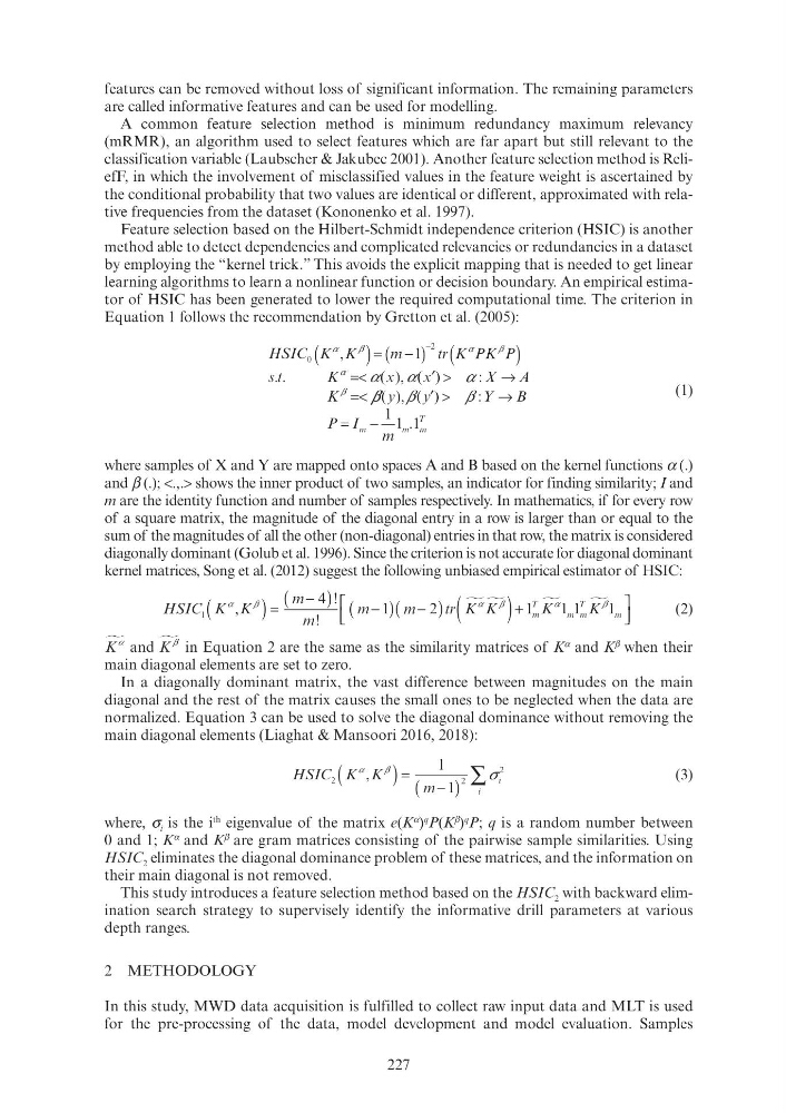
Feature selection based on the Hilbert-Schmidt independence criterion (HSIC) is another
method able to detect dependencies and complicated relevancies or redundancies in a dataset
by employing the “kernel trick.” This avoids the explicit mapping that is needed to get linear
learning algorithms to learn a nonlinear function or decision boundary. An empirical estimator of HSIC has been generated to lower the required computational time. The criterion in
Equation 1 follows the recommendation by Gretton et al. (2005):
tr
s t
K
x
X
A
K
0
C C
2
α
β
α
. .
t
( )
α x , (
α α )
:
α
(
)
K K
α
β
K
,
= (
)
m 1
m
(
)
K PK P
α
β
PK
→
X
:
α
=<
′
−
β
β
β β
β
β β β β
(
β )
:
β
.
y
β (
β
Y
B
P I
m
m
m
I
m
T
′
→
:
β Y
−
I
1 1 1
.
m
(1)
where samples of X and Y are mapped onto spaces A and B based on the kernel functions α (.)
and β (.); <.,.> shows the inner product of two samples, an indicator for finding similarity; I and
m are the identity function and number of samples respectively. In mathematics, if for every row
of a square matrix, the magnitude of the diagonal entry in a row is larger than or equal to the
sum of the magnitudes of all the other (non-diagonal) entries in that row, the matrix is considered
diagonally dominant (Golub et al. 1996). Since the criterion is not accurate for diagonal dominant
kernel matrices, Song et al. (2012) suggest the following unbiased empirical estimator of HSIC:
HSIC K K
m
tr K K
m
T
m m
m
1
C C
1
1
K
m
T
1
K
α
β
K
α
β
K
α
β
T
1 1 K
T
,
!
!
(
) = (
)
m 4
−
(
)
m 1 (
)
m 2
m
( ) +
⎡ ⎡
⎣
⎡ ⎡ ⎡ ⎡ ⎡ ⎡ ⎡ ⎡
⎣ ⎣
⎡ ⎡ ⎡ ⎡ ⎡ ⎡ ⎡
⎤
⎦
⎤ ⎤ ⎤
⎦ ⎦
⎤ ⎤ ⎤ ⎤
(2)
K
α
and K
β
in Equation 2 are the same as the similarity matrices of K
α and K
β when their
main diagonal elements are set to zero.
In a diagonally dominant matrix, the vast difference between magnitudes on the main
diagonal and the rest of the matrix causes the small ones to be neglected when the data are
normalized. Equation 3 can be used to solve the diagonal dominance without removing the
main diagonal elements (Liaghat & Mansoori 2016, 2018):
HSIC K K
i
i
2
C C
2
2
1
α
β
K
σ i
2 2
,
(
) = ( )
m 1
−
∑
(3)
where, σ i is the i
th eigenvalue of the matrix e(K
α )
q
P(K
β
)
q
P; q is a random number between
0 and 1; K
α and K
β are gram matrices consisting of the pairwise sample similarities. Using
HSIC 2 eliminates the diagonal dominance problem of these matrices, and the information on
their main diagonal is not removed.
This study introduces a feature selection method based on the HSIC 2 with backward elimination search strategy to supervisely identify the informative drill parameters at various
depth ranges.
2 METHODOLOGY
In this study, MWD data acquisition is fulfilled to collect raw input data and MLT is used
for the pre-processing of the data, model development and model evaluation. Samples
features can be removed without loss of significant information. The remaining parameters
are called informative features and can be used for modelling.
A common feature selection method is minimum redundancy maximum relevancy
(mRMR), an algorithm used to select features which are far apart but still relevant to the
classification variable (Laubscher & Jakubec 2001). Another feature selection method is ReliefF, in which the involvement of misclassified values in the feature weight is ascertained by
the conditional probability that two values are identical or different, approximated with relative frequencies from the dataset (Kononenko et al. 1997).
Feature selection based on the Hilbert-Schmidt independence criterion (HSIC) is another
method able to detect dependencies and complicated relevancies or redundancies in a dataset
by employing the “kernel trick.” This avoids the explicit mapping that is needed to get linear
learning algorithms to learn a nonlinear function or decision boundary. An empirical estimator of HSIC has been generated to lower the required computational time. The criterion in
Equation 1 follows the recommendation by Gretton et al. (2005):
tr
s t
K
x
X
A
K
0
C C
2
α
β
α
. .
t
( )
α x , (
α α )
:
α
(
)
K K
α
β
K
,
= (
)
m 1
m
(
)
K PK P
α
β
PK
→
X
:
α
=<
′
−
β
β
β β
β
β β β β
(
β )
:
β
.
y
β (
β
Y
B
P I
m
m
m
I
m
T
′
→
:
β Y
−
I
1 1 1
.
m
(1)
where samples of X and Y are mapped onto spaces A and B based on the kernel functions α (.)
and β (.); <.,.> shows the inner product of two samples, an indicator for finding similarity; I and
m are the identity function and number of samples respectively. In mathematics, if for every row
of a square matrix, the magnitude of the diagonal entry in a row is larger than or equal to the
sum of the magnitudes of all the other (non-diagonal) entries in that row, the matrix is considered
diagonally dominant (Golub et al. 1996). Since the criterion is not accurate for diagonal dominant
kernel matrices, Song et al. (2012) suggest the following unbiased empirical estimator of HSIC:
HSIC K K
m
tr K K
m
T
m m
m
1
C C
1
1
K
m
T
1
K
α
β
K
α
β
K
α
β
T
1 1 K
T
,
!
!
(
) = (
)
m 4
−
(
)
m 1 (
)
m 2
m
( ) +
⎡ ⎡
⎣
⎡ ⎡ ⎡ ⎡ ⎡ ⎡ ⎡ ⎡
⎣ ⎣
⎡ ⎡ ⎡ ⎡ ⎡ ⎡ ⎡
⎤
⎦
⎤ ⎤ ⎤
⎦ ⎦
⎤ ⎤ ⎤ ⎤
(2)
K
α
and K
β
in Equation 2 are the same as the similarity matrices of K
α and K
β when their
main diagonal elements are set to zero.
In a diagonally dominant matrix, the vast difference between magnitudes on the main
diagonal and the rest of the matrix causes the small ones to be neglected when the data are
normalized. Equation 3 can be used to solve the diagonal dominance without removing the
main diagonal elements (Liaghat & Mansoori 2016, 2018):
HSIC K K
i
i
2
C C
2
2
1
α
β
K
σ i
2 2
,
(
) = ( )
m 1
−
∑
(3)
where, σ i is the i
th eigenvalue of the matrix e(K
α )
q
P(K
β
)
q
P; q is a random number between
0 and 1; K
α and K
β are gram matrices consisting of the pairwise sample similarities. Using
HSIC 2 eliminates the diagonal dominance problem of these matrices, and the information on
their main diagonal is not removed.
This study introduces a feature selection method based on the HSIC 2 with backward elimination search strategy to supervisely identify the informative drill parameters at various
depth ranges.
2 METHODOLOGY
In this study, MWD data acquisition is fulfilled to collect raw input data and MLT is used
for the pre-processing of the data, model development and model evaluation. Samples