

169
CNNs are a natural extension of neural networks to inputs in a grid-like topology. Usually, the nature of inputs vary from temporal 1D/2D data, RGB images (3D) and Videos
(4D) while the nature of outputs are either a probability vector, for classification tasks, or a
continuous vector, for regression problems.
Their main feature of sharing inner parameters across the network leads to architectural
properties of scale, shift and distortion invariance, making them a powerful tool for image
feature extraction. Those properties mean that regardless where and how a specific raw feature appears in the image, a suitable and well-trained CNN is able to capture that feature.
Once features are extracted, images can be classified, segmented or even reconstructed.
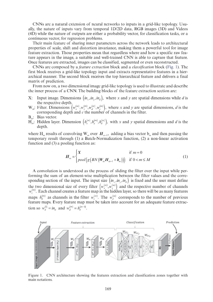
CNNs are composed by a feature extraction block and a classification block (Fig. 1). The
first block receives a grid-like topology input and extracts representative features in a hierarchical manner. The second block receives the top hierarchical feature and delivers a final
matrix of prediction.
From now on, a two dimensional image grid-like topology is used to illustrate and describe
the inner process of a CNN. The building blocks of the feature extraction section are:
X: Input image. Dimensions in in in
x
y
d
, ,
in y
in
,
(
) where x and y are spatial dimensions while d is
the respective depth.
W m : Filter. Dimensions (
)
w w w w
x
y
d
c
( )
m
( )
m
( )
m
( )
m
w w
w w
y
d
, where x and y are spatial dimensions, d is the
corresponding depth and c the number of channels in the filter.
B m : Bias vector.
H m : Hidden layer. Dimension (
)
h h h
x
h
y
d
h
( )
m
( )
m
( )
m
h h y
h
, with x and y spatial dimensions and d is the
depth.
where H m results of convolving W m over H m−1 , adding a bias vector b m and then passing the
temporary result through (1) a Batch-Normalization function, (2) a non-linear activation
function and (3) a pooling function as:
H
X
m
m
pool
m M
=
=
(
)
g (
)
BN (
)
W H
b
m
m
m
W H
b
m
m
W H
W
m
b
≤
m
⎧
⎨
⎪ ⎧ ⎧
⎨ ⎨
⎩ ⎪
⎨ ⎨
⎩ ⎩
if
if
0
0
(1)
A convolution is understood as the process of sliding the filter over the input while performing the sum of an element-wise multiplication between the filter values and the corresponding section of the input. The input size in in in
x
y
d
, ,
in y
in
(
) is fixed and the user must define
the two dimensional size of every filter (
)
(
w w
x
y
( )
m
( )
m
and the respective number of channels
w c
( )
m . Each channel creates a feature map in the hidden layer, so there will be as many features
maps h d
h
( )
m as channels in the filter w c
( )
m . The w d
( )
m corresponds to the number of previous
feature maps. Every feature map must be taken into account for an adequate feature extraction so w
in
i
d
d
in i i
( )
1
and w
h
d
d
h
( )
m
( )
m − .
Figure 1. CNN architecture showing the features extraction and classification zones together with
main notations.
Feature extraction
Classification
CNNs are a natural extension of neural networks to inputs in a grid-like topology. Usually, the nature of inputs vary from temporal 1D/2D data, RGB images (3D) and Videos
(4D) while the nature of outputs are either a probability vector, for classification tasks, or a
continuous vector, for regression problems.
Their main feature of sharing inner parameters across the network leads to architectural
properties of scale, shift and distortion invariance, making them a powerful tool for image
feature extraction. Those properties mean that regardless where and how a specific raw feature appears in the image, a suitable and well-trained CNN is able to capture that feature.
Once features are extracted, images can be classified, segmented or even reconstructed.
CNNs are composed by a feature extraction block and a classification block (Fig. 1). The
first block receives a grid-like topology input and extracts representative features in a hierarchical manner. The second block receives the top hierarchical feature and delivers a final
matrix of prediction.
From now on, a two dimensional image grid-like topology is used to illustrate and describe
the inner process of a CNN. The building blocks of the feature extraction section are:
X: Input image. Dimensions in in in
x
y
d
, ,
in y
in
,
(
) where x and y are spatial dimensions while d is
the respective depth.
W m : Filter. Dimensions (
)
w w w w
x
y
d
c
( )
m
( )
m
( )
m
( )
m
w w
w w
y
d
, where x and y are spatial dimensions, d is the
corresponding depth and c the number of channels in the filter.
B m : Bias vector.
H m : Hidden layer. Dimension (
)
h h h
x
h
y
d
h
( )
m
( )
m
( )
m
h h y
h
, with x and y spatial dimensions and d is the
depth.
where H m results of convolving W m over H m−1 , adding a bias vector b m and then passing the
temporary result through (1) a Batch-Normalization function, (2) a non-linear activation
function and (3) a pooling function as:
H
X
m
m
pool
m M
=
=
(
)
g (
)
BN (
)
W H
b
m
m
m
W H
b
m
m
W H
W
m
b
≤
m
⎧
⎨
⎪ ⎧ ⎧
⎨ ⎨
⎩ ⎪
⎨ ⎨
⎩ ⎩
if
if
0
0
(1)
A convolution is understood as the process of sliding the filter over the input while performing the sum of an element-wise multiplication between the filter values and the corresponding section of the input. The input size in in in
x
y
d
, ,
in y
in
(
) is fixed and the user must define
the two dimensional size of every filter (
)
(
w w
x
y
( )
m
( )
m
and the respective number of channels
w c
( )
m . Each channel creates a feature map in the hidden layer, so there will be as many features
maps h d
h
( )
m as channels in the filter w c
( )
m . The w d
( )
m corresponds to the number of previous
feature maps. Every feature map must be taken into account for an adequate feature extraction so w
in
i
d
d
in i i
( )
1
and w
h
d
d
h
( )
m
( )
m − .
Figure 1. CNN architecture showing the features extraction and classification zones together with
main notations.
Feature extraction
Classification