

159
the secondary variable, which represents more availability, is of paramount importance for
estimation of primary variable, particularly if there exist an interdependency characteristics
between them. Hierarchical cokriging procedure, in this paper, introduces an innovative
algorithm to estimate the variables in turn, rather than simultaneously. This methodology
integrates multi-collocated cokriging to estimate the primary variable beyond the secondary variables that is estimated beforehand in hierarchical sequence. The goal of this paper is
threefold: First, it is of interest to provide a background about the co-estimation methodologies, theory behind and the algorithm proposed. Second, a real case study is presented from
a copper deposit that gold grade as the primary variable is estimated, based on the proposed
algorithm, condition to the primary variable, copper grade which already estimated. Last,
the results are then compared with traditional cokriging approaches and relevant discussion
is provided as conclusion.
2 METHODOLOGY
2.1 Ordinary cokriging system
Ordinary cokriging is an extension of ordinary kriging, allows predication of primary and
secondary variable by taking into account their cross-correlated structures (Wackernagel,
2003; Chilès and Delfiner, 2012). Stationary characteristics of mean values are restricted to
a local neighborhood centered on the location x being estimated. The ordinary cokriging
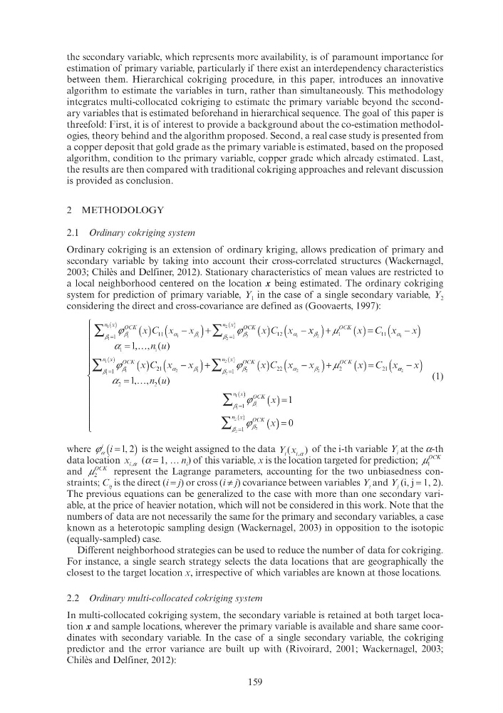
system for prediction of primary variable, Y 1 in the case of a single secondary variable, Y 2
considering the direct and cross-covariance are defined as (Goovaerts, 1997):
ϕ
β
β
β
β
1
1
β β
2
β β
2
β β
2
1
1
12
n
OC
ϕ
K
C C
n 2
C 1
=
( )
x
=
( )
x
∑
∑
ϕ β
ϕ ϕ
β
1
β
1
1
11
OC
ϕ
K
C
n 1
C
=
( )
x
( ) (
)
1
1
β
α
1
α
β
α
( )
x
C
n
C
OCK C C
OCK C C
n
β
β
μ
O
α
ϕ
O
1
β β
1
β β
1
C C
1
1
n
α α
1
1
(
)
α 1
α α
x − x x x β 2
β β
+
( )
x x x = C C C (
)
x
x
α
x
1
α α −
x x
= 1
( )
x
=
( )
x
∑
( )
u
21
C 2 2
C C C C
1
22
2
2 1
2
2
2
C
C 2
OCK C
n 2
OCK C C
β 2
β 2 2
μ 2 2
O
22
C 2
ϕ
2
OCK C C
β 2 2
(
)
2
1
x
x
α
β
2
1
1
x +
( )
x
(
)
2
2
α 2
2
(
)
2
x
x
α
β
2
2
2
x +
( )
x
=
( )
x
∑
β
β
β
β
α
ϕ
ϕ
1
β β
1
β β
1
2
β β
2
β β
2
2
2
α α
1
1
1
1
(
)
x α α 2
α α −
= 1
( ) =
(
=
( )
=
( )
∑
∑
n 2
x
OC
ϕ
K
C C
n 1 1 (
OC
ϕ
K
C C
n 2 (
( )
u
) ) =
⎧
⎨
⎪
⎧ ⎧
⎪
⎪ ⎪
⎪
⎪ ⎪
⎪
⎪ ⎪
⎪
⎨ ⎨
⎪ ⎪
⎩
⎪
⎨ ⎨
⎪
⎪ ⎪
⎪
⎪ ⎪
⎪
⎪ ⎪
⎪ ⎩ ⎩
⎪ ⎪
0
(1)
where ϕ α
i
ϕ ϕ (
)
i =
is the weight assigned to the data Y i i
Y Y ( )
x i
x ,α of the i-th variable Y i at the α-th
data location x i,α (α = 1, … n i ) of this variable, x is the location targeted for prediction; μ 1
μ μ
OC
μ μ
K
C C
and μ 2
μ
OC
μ μ
K
C C
represent the Lagrange parameters, accounting for the two unbiasedness constraints; C ij is the direct (i = j) or cross (i ≠ j) covariance between variables Y i and Y j (i, j = 1, 2).
The previous equations can be generalized to the case with more than one secondary variable, at the price of heavier notation, which will not be considered in this work. Note that the
numbers of data are not necessarily the same for the primary and secondary variables, a case
known as a heterotopic sampling design (Wackernagel, 2003) in opposition to the isotopic
(equally-sampled) case.
Different neighborhood strategies can be used to reduce the number of data for cokriging.
For instance, a single search strategy selects the data locations that are geographically the
closest to the target location x, irrespective of which variables are known at those locations.
2.2 Ordinary multi-collocated cokriging system
In multi-collocated cokriging system, the secondary variable is retained at both target location x and sample locations, wherever the primary variable is available and share same coordinates with secondary variable. In the case of a single secondary variable, the cokriging
predictor and the error variance are built up with (Rivoirard, 2001; Wackernagel, 2003;
Chilès and Delfiner, 2012):
the secondary variable, which represents more availability, is of paramount importance for
estimation of primary variable, particularly if there exist an interdependency characteristics
between them. Hierarchical cokriging procedure, in this paper, introduces an innovative
algorithm to estimate the variables in turn, rather than simultaneously. This methodology
integrates multi-collocated cokriging to estimate the primary variable beyond the secondary variables that is estimated beforehand in hierarchical sequence. The goal of this paper is
threefold: First, it is of interest to provide a background about the co-estimation methodologies, theory behind and the algorithm proposed. Second, a real case study is presented from
a copper deposit that gold grade as the primary variable is estimated, based on the proposed
algorithm, condition to the primary variable, copper grade which already estimated. Last,
the results are then compared with traditional cokriging approaches and relevant discussion
is provided as conclusion.
2 METHODOLOGY
2.1 Ordinary cokriging system
Ordinary cokriging is an extension of ordinary kriging, allows predication of primary and
secondary variable by taking into account their cross-correlated structures (Wackernagel,
2003; Chilès and Delfiner, 2012). Stationary characteristics of mean values are restricted to
a local neighborhood centered on the location x being estimated. The ordinary cokriging
system for prediction of primary variable, Y 1 in the case of a single secondary variable, Y 2
considering the direct and cross-covariance are defined as (Goovaerts, 1997):
ϕ
β
β
β
β
1
1
β β
2
β β
2
β β
2
1
1
12
n
OC
ϕ
K
C C
n 2
C 1
=
( )
x
=
( )
x
∑
∑
ϕ β
ϕ ϕ
β
1
β
1
1
11
OC
ϕ
K
C
n 1
C
=
( )
x
( ) (
)
1
1
β
α
1
α
β
α
( )
x
C
n
C
OCK C C
OCK C C
n
β
β
μ
O
α
ϕ
O
1
β β
1
β β
1
C C
1
1
n
α α
1
1
(
)
α 1
α α
x − x x x β 2
β β
+
( )
x x x = C C C (
)
x
x
α
x
1
α α −
x x
= 1
( )
x
=
( )
x
∑
( )
u
21
C 2 2
C C C C
1
22
2
2 1
2
2
2
C
C 2
OCK C
n 2
OCK C C
β 2
β 2 2
μ 2 2
O
22
C 2
ϕ
2
OCK C C
β 2 2
(
)
2
1
x
x
α
β
2
1
1
x +
( )
x
(
)
2
2
α 2
2
(
)
2
x
x
α
β
2
2
2
x +
( )
x
=
( )
x
∑
β
β
β
β
α
ϕ
ϕ
1
β β
1
β β
1
2
β β
2
β β
2
2
2
α α
1
1
1
1
(
)
x α α 2
α α −
= 1
( ) =
(
=
( )
=
( )
∑
∑
n 2
x
OC
ϕ
K
C C
n 1 1 (
OC
ϕ
K
C C
n 2 (
( )
u
) ) =
⎧
⎨
⎪
⎧ ⎧
⎪
⎪ ⎪
⎪
⎪ ⎪
⎪
⎪ ⎪
⎪
⎨ ⎨
⎪ ⎪
⎩
⎪
⎨ ⎨
⎪
⎪ ⎪
⎪
⎪ ⎪
⎪
⎪ ⎪
⎪ ⎩ ⎩
⎪ ⎪
0
(1)
where ϕ α
i
ϕ ϕ (
)
i =
is the weight assigned to the data Y i i
Y Y ( )
x i
x ,α of the i-th variable Y i at the α-th
data location x i,α (α = 1, … n i ) of this variable, x is the location targeted for prediction; μ 1
μ μ
OC
μ μ
K
C C
and μ 2
μ
OC
μ μ
K
C C
represent the Lagrange parameters, accounting for the two unbiasedness constraints; C ij is the direct (i = j) or cross (i ≠ j) covariance between variables Y i and Y j (i, j = 1, 2).
The previous equations can be generalized to the case with more than one secondary variable, at the price of heavier notation, which will not be considered in this work. Note that the
numbers of data are not necessarily the same for the primary and secondary variables, a case
known as a heterotopic sampling design (Wackernagel, 2003) in opposition to the isotopic
(equally-sampled) case.
Different neighborhood strategies can be used to reduce the number of data for cokriging.
For instance, a single search strategy selects the data locations that are geographically the
closest to the target location x, irrespective of which variables are known at those locations.
2.2 Ordinary multi-collocated cokriging system
In multi-collocated cokriging system, the secondary variable is retained at both target location x and sample locations, wherever the primary variable is available and share same coordinates with secondary variable. In the case of a single secondary variable, the cokriging
predictor and the error variance are built up with (Rivoirard, 2001; Wackernagel, 2003;
Chilès and Delfiner, 2012):