

111
The methodology can be used as a fully automatic workflow. However, human interaction with a spatial continuity model may be useful, because it can provide interpretation
and uncertainty analysis if desired. A possible input from the geo-modeler is to impose a
preferential direction when building the BMEC. The CT extracted from it will reproduce
those anisotropy directions. Another potential problem is the size of the CT. For a very large
area, or even inclined boreholes, the CT requires to compute covariances for all distances. An
analytic form of covariance is needed for those cases.
5 CASE STUDY
For the case study, a three dimensional multivariate data set from an iron deposit in Brazil
was used. However, due to the extension of the data set it was chosen to work with the two
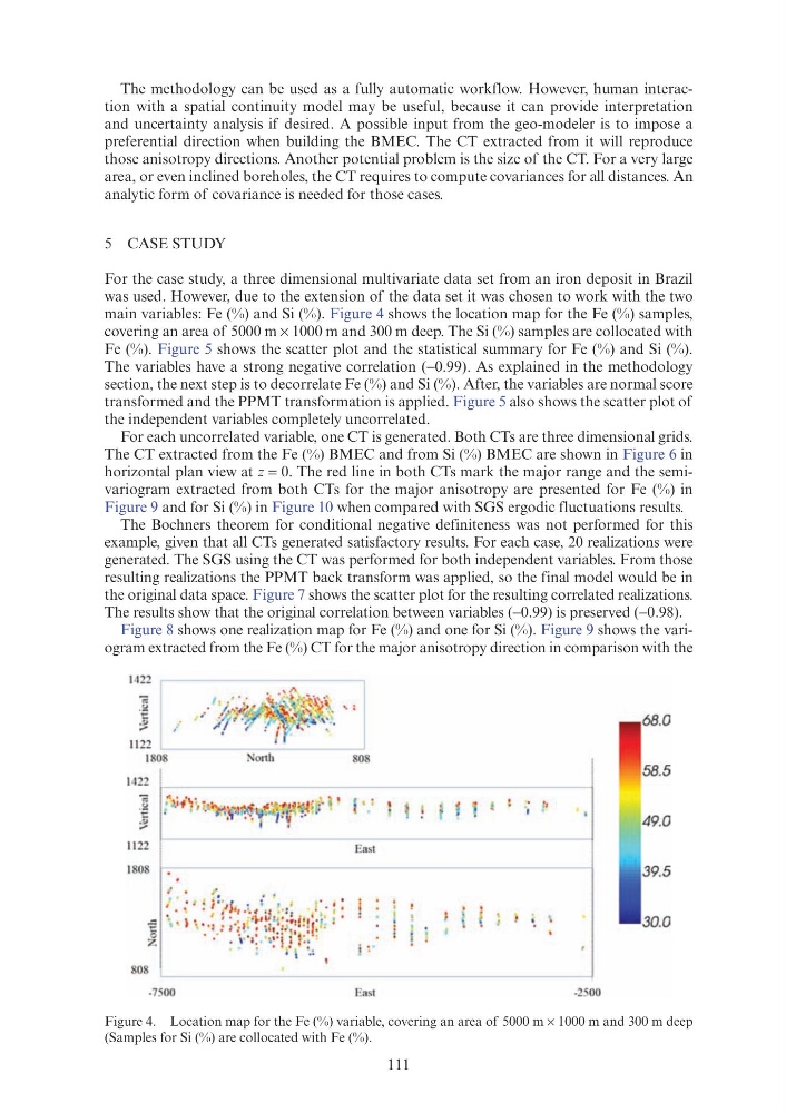
main variables: Fe (%) and Si (%). Figure 4 shows the location map for the Fe (%) samples,
covering an area of 5000 m × 1000 m and 300 m deep. The Si (%) samples are collocated with
Fe (%). Figure 5 shows the scatter plot and the statistical summary for Fe (%) and Si (%).
The variables have a strong negative correlation (−0.99). As explained in the methodology
section, the next step is to decorrelate Fe (%) and Si (%). After, the variables are normal score
transformed and the PPMT transformation is applied. Figure 5 also shows the scatter plot of
the independent variables completely uncorrelated.
For each uncorrelated variable, one CT is generated. Both CTs are three dimensional grids.
The CT extracted from the Fe (%) BMEC and from Si (%) BMEC are shown in Figure 6 in
horizontal plan view at z = 0. The red line in both CTs mark the major range and the semivariogram extracted from both CTs for the major anisotropy are presented for Fe (%) in
Figure 9 and for Si (%) in Figure 10 when compared with SGS ergodic fluctuations results.
The Bochners theorem for conditional negative definiteness was not performed for this
example, given that all CTs generated satisfactory results. For each case, 20 realizations were
generated. The SGS using the CT was performed for both independent variables. From those
resulting realizations the PPMT back transform was applied, so the final model would be in
the original data space. Figure 7 shows the scatter plot for the resulting correlated realizations.
The results show that the original correlation between variables (−0.99) is preserved (−0.98).
Figure 8 shows one realization map for Fe (%) and one for Si (%). Figure 9 shows the variogram extracted from the Fe (%) CT for the major anisotropy direction in comparison with the
Figure 4. Location map for the Fe (%) variable, covering an area of 5000 m × 1000 m and 300 m deep
(Samples for Si (%) are collocated with Fe (%).
68.0
58.5
I I
49.0
East
1808
39.5
'
I
I
30.0
-7500
East
-2500
The methodology can be used as a fully automatic workflow. However, human interaction with a spatial continuity model may be useful, because it can provide interpretation
and uncertainty analysis if desired. A possible input from the geo-modeler is to impose a
preferential direction when building the BMEC. The CT extracted from it will reproduce
those anisotropy directions. Another potential problem is the size of the CT. For a very large
area, or even inclined boreholes, the CT requires to compute covariances for all distances. An
analytic form of covariance is needed for those cases.
5 CASE STUDY
For the case study, a three dimensional multivariate data set from an iron deposit in Brazil
was used. However, due to the extension of the data set it was chosen to work with the two
main variables: Fe (%) and Si (%). Figure 4 shows the location map for the Fe (%) samples,
covering an area of 5000 m × 1000 m and 300 m deep. The Si (%) samples are collocated with
Fe (%). Figure 5 shows the scatter plot and the statistical summary for Fe (%) and Si (%).
The variables have a strong negative correlation (−0.99). As explained in the methodology
section, the next step is to decorrelate Fe (%) and Si (%). After, the variables are normal score
transformed and the PPMT transformation is applied. Figure 5 also shows the scatter plot of
the independent variables completely uncorrelated.
For each uncorrelated variable, one CT is generated. Both CTs are three dimensional grids.
The CT extracted from the Fe (%) BMEC and from Si (%) BMEC are shown in Figure 6 in
horizontal plan view at z = 0. The red line in both CTs mark the major range and the semivariogram extracted from both CTs for the major anisotropy are presented for Fe (%) in
Figure 9 and for Si (%) in Figure 10 when compared with SGS ergodic fluctuations results.
The Bochners theorem for conditional negative definiteness was not performed for this
example, given that all CTs generated satisfactory results. For each case, 20 realizations were
generated. The SGS using the CT was performed for both independent variables. From those
resulting realizations the PPMT back transform was applied, so the final model would be in
the original data space. Figure 7 shows the scatter plot for the resulting correlated realizations.
The results show that the original correlation between variables (−0.99) is preserved (−0.98).
Figure 8 shows one realization map for Fe (%) and one for Si (%). Figure 9 shows the variogram extracted from the Fe (%) CT for the major anisotropy direction in comparison with the
Figure 4. Location map for the Fe (%) variable, covering an area of 5000 m × 1000 m and 300 m deep
(Samples for Si (%) are collocated with Fe (%).
68.0
58.5
I I
49.0
East
1808
39.5
'
I
I
30.0
-7500
East
-2500