

Theor Chem Acc (2015) 134:86
1 3
P and of the fi rst- and second-order density matrices,
respectively:
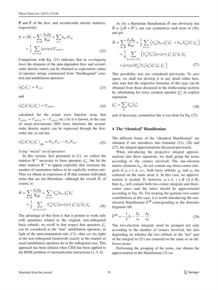
Comparison with Eq. ( 21 ) indicates that in overlapping
basis the elements of the spin-dependent fi rst- and secondorder density matrix can be obtained as expectation values
of operator strings constructed from “biorthogonal” creation and annihilation operators:
and
calculated for the actual wave function (note that
κρμν = ρκνμ = − ρκμν etc.) As it is known, in the case
of single-determinant (SD) wave functions the secondorder density matrix can be expressed through the fi rstorder one, so one has
Using “mixed” set of operators
In this version, fi rst presented in [ 1 ], we collect the
matrices S −1 necessary to form operators ˆ
ϕ −
μ , but let the
other matrices S −1 to appear explicitly (this increases the
number of summation indices to be explicitly written out).
Thus we obtain an expression of ˆ
H that contains individual
terms that are not Hermitian—although the overall ˆ
H , of
course, is:
The advantage of this form is that it permits to work only
with quantities related to the original, non-orthogonal
basis orbitals; we recall in that respect that operators ˆ
ϕ −
μ
can be considered as the “true” annihilation operators, in
light of the anticommutation rule ( 17 )—they act (to right)
in the non-orthogonal framework exactly in the manner as
usual annihilation operators do in the orthogonal case. This
approach has been utilized when CHA has been applied to
the BSSE problem of intermolecular interactions [ 1 , 3 , 4 ].
(22)
E = = ˆ
H =
A
R AB
+
μ,ν
h μν P νμ
+
1
2
μ,ν,κ,ρ
[μν|κρ] κρμν .
(23)
ˆ
ϕ
+
μ ˆ
ϕ
−
ν
= P νμ ;
(24)
ˆ
ϕ
+
μ ˆ
ϕ
+
ν ˆ
ϕ
−
ρ ˆ
ϕ
−
κ
= κρμν ,
(25)
ˆ
ϕ
+
μ ˆ
ϕ
+
ν ˆ
ϕ
−
ρ ˆ
ϕ
−
κ
SD
= P κμ P ρν − P κν P ρμ .
(26)
ˆ
H =
A
R AB
+
μ,ν,ρ
S
−1
ρμ h μν ˆ
χ
+
ρ ˆ
ϕ
−
ν
+
1
2
μ,ν,ρ,τ ,,σ
S
−1
μ S
−1
σ ν [μν|ρτ ] ˆ
χ
+
ˆ
χ
+
σ ˆ
ϕ
−
τ ˆ
ϕ
−
ρ
As for a Hermitian Hamiltonian ˆ
H one obviously has
ˆ
H ≡
1
2 ( ˆ
H + ˆ
H † ) , one can symmetrize each term of ( 26 ),
and get:
This possibility was not considered previously. To save
space, we shall not develop it in any detail either here,
only note that the respective formulae of this type can be
obtained from those discussed in the forthcoming sections
by substituting for every creation operator ˆ
ϕ +
μ its explicit
expansion
and, if necessary, symmetrize like it was done for Eq. ( 27 ).
4 The “chemical” Hamiltonian
The different forms of the “chemical Hamiltonian” are
obtained if one introduces into formulae ( 21 ), ( 26 ) and
( 27 ), the integral approximations discussed previously.
When introducing the projective integral approximations into these equations, we shall group the terms
according to the centers involved. The one-electron
matrix elements h μν do not contain any three-center integrals if μ, ν ∈ A , i.e., both basis orbitals χ μ and χ ν are
centered on the same atom A . In this case, no approximation is needed. If, however, μ ∈ A , ν ∈ B ( A = B ),
then h μν will contain both two-center integrals and threecenter ones—and the latter should be approximated
according to Eq. ( 8 ). For treating the genuine two-center
contributions in this case, it is worth introducing the oneelectron Hamiltonian ˆ
h AB corresponding to the diatomic
fragment AB :
The two-electron integrals need be grouped not only
according to the number of centers involved, but also
depending on whether the two orbitals in the “ket” part
of the integral in ( 21 ) are centered on the same or on different atoms.
Performing the grouping of the terms, one obtains the
approximation to the Hamiltonian ( 21 ) as
(27)
ˆ
H =
훀
A
R AB
+
1
2
μ,ν,ρ
S
−1
ρμ h μν ˆ
χ
+
ρ ˆ
ϕ
−
ν + h νμ S
−1
μρ ˆ
ϕ
+
ν ˆ
χ
−
ρ
+
1
4
μ,ν,ρ,τ ,,σ
S
−1
μ S
−1
σ ν [μν|ρτ ] ˆ
χ
+
ˆ
χ
+
σ ˆ
ϕ
−
τ ˆ
ϕ
−
ρ
+ [ρτ |μν]S
−1
μ S
−1
νσ ϕ
+
ρ ˆ
ϕ
+
τ ˆ
χ
−
σ ˆ
χ
−
(28)
ˆ
ϕ
+
ρ =
μ
S
−1
μρ ˆ
χ
+
μ .
(29)
ˆ
h
AB
= −
1
2
−
Z A
r A
−
Z B
r B
.
35
Reprinted from the journal
1 3
P and of the fi rst- and second-order density matrices,
respectively:
Comparison with Eq. ( 21 ) indicates that in overlapping
basis the elements of the spin-dependent fi rst- and secondorder density matrix can be obtained as expectation values
of operator strings constructed from “biorthogonal” creation and annihilation operators:
and
calculated for the actual wave function (note that
κρμν = ρκνμ = − ρκμν etc.) As it is known, in the case
of single-determinant (SD) wave functions the secondorder density matrix can be expressed through the fi rstorder one, so one has
Using “mixed” set of operators
In this version, fi rst presented in [ 1 ], we collect the
matrices S −1 necessary to form operators ˆ
ϕ −
μ , but let the
other matrices S −1 to appear explicitly (this increases the
number of summation indices to be explicitly written out).
Thus we obtain an expression of ˆ
H that contains individual
terms that are not Hermitian—although the overall ˆ
H , of
course, is:
The advantage of this form is that it permits to work only
with quantities related to the original, non-orthogonal
basis orbitals; we recall in that respect that operators ˆ
ϕ −
μ
can be considered as the “true” annihilation operators, in
light of the anticommutation rule ( 17 )—they act (to right)
in the non-orthogonal framework exactly in the manner as
usual annihilation operators do in the orthogonal case. This
approach has been utilized when CHA has been applied to
the BSSE problem of intermolecular interactions [ 1 , 3 , 4 ].
(22)
E = = ˆ
H =
A
R AB
+
μ,ν
h μν P νμ
+
1
2
μ,ν,κ,ρ
[μν|κρ] κρμν .
(23)
ˆ
ϕ
+
μ ˆ
ϕ
−
ν
= P νμ ;
(24)
ˆ
ϕ
+
μ ˆ
ϕ
+
ν ˆ
ϕ
−
ρ ˆ
ϕ
−
κ
= κρμν ,
(25)
ˆ
ϕ
+
μ ˆ
ϕ
+
ν ˆ
ϕ
−
ρ ˆ
ϕ
−
κ
SD
= P κμ P ρν − P κν P ρμ .
(26)
ˆ
H =
A
R AB
+
μ,ν,ρ
S
−1
ρμ h μν ˆ
χ
+
ρ ˆ
ϕ
−
ν
+
1
2
μ,ν,ρ,τ ,,σ
S
−1
μ S
−1
σ ν [μν|ρτ ] ˆ
χ
+
ˆ
χ
+
σ ˆ
ϕ
−
τ ˆ
ϕ
−
ρ
As for a Hermitian Hamiltonian ˆ
H one obviously has
ˆ
H ≡
1
2 ( ˆ
H + ˆ
H † ) , one can symmetrize each term of ( 26 ),
and get:
This possibility was not considered previously. To save
space, we shall not develop it in any detail either here,
only note that the respective formulae of this type can be
obtained from those discussed in the forthcoming sections
by substituting for every creation operator ˆ
ϕ +
μ its explicit
expansion
and, if necessary, symmetrize like it was done for Eq. ( 27 ).
4 The “chemical” Hamiltonian
The different forms of the “chemical Hamiltonian” are
obtained if one introduces into formulae ( 21 ), ( 26 ) and
( 27 ), the integral approximations discussed previously.
When introducing the projective integral approximations into these equations, we shall group the terms
according to the centers involved. The one-electron
matrix elements h μν do not contain any three-center integrals if μ, ν ∈ A , i.e., both basis orbitals χ μ and χ ν are
centered on the same atom A . In this case, no approximation is needed. If, however, μ ∈ A , ν ∈ B ( A = B ),
then h μν will contain both two-center integrals and threecenter ones—and the latter should be approximated
according to Eq. ( 8 ). For treating the genuine two-center
contributions in this case, it is worth introducing the oneelectron Hamiltonian ˆ
h AB corresponding to the diatomic
fragment AB :
The two-electron integrals need be grouped not only
according to the number of centers involved, but also
depending on whether the two orbitals in the “ket” part
of the integral in ( 21 ) are centered on the same or on different atoms.
Performing the grouping of the terms, one obtains the
approximation to the Hamiltonian ( 21 ) as
(27)
ˆ
H =
훀
A
R AB
+
1
2
μ,ν,ρ
S
−1
ρμ h μν ˆ
χ
+
ρ ˆ
ϕ
−
ν + h νμ S
−1
μρ ˆ
ϕ
+
ν ˆ
χ
−
ρ
+
1
4
μ,ν,ρ,τ ,,σ
S
−1
μ S
−1
σ ν [μν|ρτ ] ˆ
χ
+
ˆ
χ
+
σ ˆ
ϕ
−
τ ˆ
ϕ
−
ρ
+ [ρτ |μν]S
−1
μ S
−1
νσ ϕ
+
ρ ˆ
ϕ
+
τ ˆ
χ
−
σ ˆ
χ
−
(28)
ˆ
ϕ
+
ρ =
μ
S
−1
μρ ˆ
χ
+
μ .
(29)
ˆ
h
AB
= −
1
2
−
Z A
r A
−
Z B
r B
.
35
Reprinted from the journal