

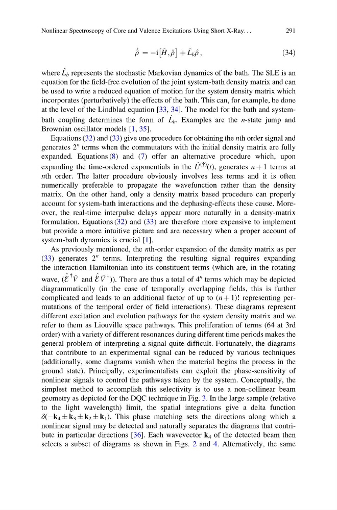
_
^
ρ ¼ Ài ^
H; ^
ρ
Â
à þ ^
L b ^
ρ ;
ð34Þ
where ^
L b represents the stochastic Markovian dynamics of the bath. The SLE is an
equation for the field-free evolution of the joint system-bath density matrix and can
be used to write a reduced equation of motion for the system density matrix which
incorporates (perturbatively) the effects of the bath. This can, for example, be done
at the level of the Lindblad equation [33, 34]. The model for the bath and systembath coupling determines the form of ^
L b . Examples are the n-state jump and
Brownian oscillator models [1, 35].
Equations (32) and (33) give one procedure for obtaining the nth order signal and
generates 2
n terms when the commutators with the initial density matrix are fully
expanded. Equations (8) and (7) offer an alternative procedure which, upon
expanding the time-ordered exponentials in the ^
U
({) (t), generates n þ 1 terms at
nth order. The latter procedure obviously involves less terms and it is often
numerically preferable to propagate the wavefunction rather than the density
matrix. On the other hand, only a density matrix based procedure can properly
account for system-bath interactions and the dephasing-effects these cause. Moreover, the real-time interpulse delays appear more naturally in a density-matrix
formulation. Equations (32) and (33) are therefore more expensive to implement
but provide a more intuitive picture and are necessary when a proper account of
system-bath dynamics is crucial [1].
As previously mentioned, the nth-order expansion of the density matrix as per
(33) generates 2
n terms. Interpreting the resulting signal requires expanding
the interaction Hamiltonian into its constituent terms (which are, in the rotating
wave, ( ^
ℰ
{
^
V and ^
ℰ ^
V
{ )). There are thus a total of 4
n terms which may be depicted
diagrammatically (in the case of temporally overlapping fields, this is further
complicated and leads to an additional factor of up to (n þ 1)! representing permutations of the temporal order of field interactions). These diagrams represent
different excitation and evolution pathways for the system density matrix and we
refer to them as Liouville space pathways. This proliferation of terms (64 at 3rd
order) with a variety of different resonances during different time periods makes the
general problem of interpreting a signal quite difficult. Fortunately, the diagrams
that contribute to an experimental signal can be reduced by various techniques
(additionally, some diagrams vanish when the material begins the process in the
ground state). Principally, experimentalists can exploit the phase-sensitivity of
nonlinear signals to control the pathways taken by the system. Conceptually, the
simplest method to accomplish this selectivity is to use a non-collinear beam
geometry as depicted for the DQC technique in Fig. 3. In the large sample (relative
to the light wavelength) limit, the spatial integrations give a delta function
δ(Àk 4 Æ k 3 Æ k 2 Æ k 1 ). This phase matching sets the directions along which a
nonlinear signal may be detected and naturally separates the diagrams that contribute in particular directions [36]. Each wavevector k 4 of the detected beam then
selects a subset of diagrams as shown in Figs. 2 and 4. Alternatively, the same
Nonlinear Spectroscopy of Core and Valence Excitations Using Short X-Ray. . .
291
^
ρ ¼ Ài ^
H; ^
ρ
Â
à þ ^
L b ^
ρ ;
ð34Þ
where ^
L b represents the stochastic Markovian dynamics of the bath. The SLE is an
equation for the field-free evolution of the joint system-bath density matrix and can
be used to write a reduced equation of motion for the system density matrix which
incorporates (perturbatively) the effects of the bath. This can, for example, be done
at the level of the Lindblad equation [33, 34]. The model for the bath and systembath coupling determines the form of ^
L b . Examples are the n-state jump and
Brownian oscillator models [1, 35].
Equations (32) and (33) give one procedure for obtaining the nth order signal and
generates 2
n terms when the commutators with the initial density matrix are fully
expanded. Equations (8) and (7) offer an alternative procedure which, upon
expanding the time-ordered exponentials in the ^
U
({) (t), generates n þ 1 terms at
nth order. The latter procedure obviously involves less terms and it is often
numerically preferable to propagate the wavefunction rather than the density
matrix. On the other hand, only a density matrix based procedure can properly
account for system-bath interactions and the dephasing-effects these cause. Moreover, the real-time interpulse delays appear more naturally in a density-matrix
formulation. Equations (32) and (33) are therefore more expensive to implement
but provide a more intuitive picture and are necessary when a proper account of
system-bath dynamics is crucial [1].
As previously mentioned, the nth-order expansion of the density matrix as per
(33) generates 2
n terms. Interpreting the resulting signal requires expanding
the interaction Hamiltonian into its constituent terms (which are, in the rotating
wave, ( ^
ℰ
{
^
V and ^
ℰ ^
V
{ )). There are thus a total of 4
n terms which may be depicted
diagrammatically (in the case of temporally overlapping fields, this is further
complicated and leads to an additional factor of up to (n þ 1)! representing permutations of the temporal order of field interactions). These diagrams represent
different excitation and evolution pathways for the system density matrix and we
refer to them as Liouville space pathways. This proliferation of terms (64 at 3rd
order) with a variety of different resonances during different time periods makes the
general problem of interpreting a signal quite difficult. Fortunately, the diagrams
that contribute to an experimental signal can be reduced by various techniques
(additionally, some diagrams vanish when the material begins the process in the
ground state). Principally, experimentalists can exploit the phase-sensitivity of
nonlinear signals to control the pathways taken by the system. Conceptually, the
simplest method to accomplish this selectivity is to use a non-collinear beam
geometry as depicted for the DQC technique in Fig. 3. In the large sample (relative
to the light wavelength) limit, the spatial integrations give a delta function
δ(Àk 4 Æ k 3 Æ k 2 Æ k 1 ). This phase matching sets the directions along which a
nonlinear signal may be detected and naturally separates the diagrams that contribute in particular directions [36]. Each wavevector k 4 of the detected beam then
selects a subset of diagrams as shown in Figs. 2 and 4. Alternatively, the same
Nonlinear Spectroscopy of Core and Valence Excitations Using Short X-Ray. . .
291