

tax credits, etc., so as to be able to determine the actual cash flow every year. Even
if done on a constant-dollar basis, the annual cash flows can be expected to vary
from year to year. A discounted cash flow analysis can easily keep track of such
variations. Again, for simplicity, the concept can be explained equally well if we
assume a uniform stream of cash flows.
It is helpful to visualize expenses and cash flows as a series of arrows: positive
arrows for positive cash flows (net inflows) and negative arrows for outflows such
as capital investment and negative cash flows. We start with a fully capitalized
investment figure at time zero, the start of production.
Let n be the total number of periods. For simplicity, let us assume that n are years
and that we consider either 10 or 20 years.
Let I represent the initial investment at time zero and CF the annual cash flow
that is assumed uniform on a constant-dollar basis (i.e., no inflation).
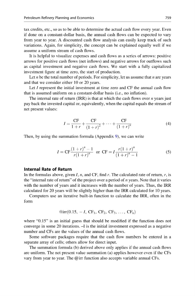
The internal rate of return (IRR) is that at which the cash flows over n years just
pay back the invested capital or, equivalently, when the capital equals the stream of
net present values:
I ¼
CF
1 þ r
þ
CF
1 þ r
ð
Þ
2
þ Á Á Á þ
CF
1 þ r
ð
Þ
n
(4)
Then, by using the summation formula (Appendix 9), we can write
I ¼ CF
1 þ r
ð
Þ
n À 1
r 1 þ r
ð
Þ
n
or CF ¼ I
r 1 þ r
ð
Þ
n
1 þ r
ð
Þ
n À 1
(5)
Internal Rate of Return
In the formulas above, given I, n, and CF, find r. The calculated rate of return, r, is
the “internal rate of return” of the project over a period of n years. Note that it varies
with the number of years and it increases with the number of years. Thus, the IRR
calculated for 20 years will be slightly higher than the IRR calculated for 10 years.
Computers use an iterative built-in function to calculate the IRR, often in the
form
@irr 0:15, À I, CF 1 , CF 2 , CF 3 , . . . , CF n
ð
Þ
where “0.15” is an initial guess that should be modified if the function does not
converge in some 20 iterations. –I is the initial investment expressed as a negative
number and CFs are the values of the annual cash flows.
Some software packages require that the cash flow numbers be entered in a
separate array of cells; others allow for direct input.
The summation formula (b) derived above only applies if the annual cash flows
are uniform. The net present value summation (a) applies however even if the CFs
vary from year to year. The @irr function also accepts variable annual CFs.
Petroleum Refinery Planning and Economics
759