

344 Appendix 2: Product Upgrades Based on Minimum Expected Quality Loss
After solving Equations A2.9 and A2.10, we obtain the following results:
C = C s m
4
l
, C = −2C s m
2
b
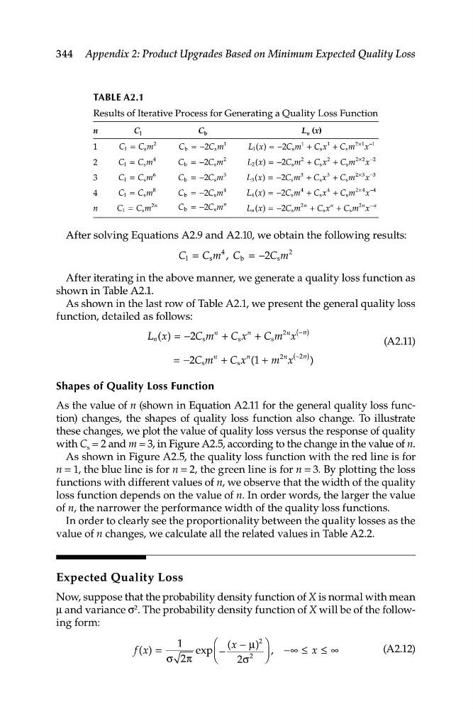
After iterating in the above manner, we generate a quality loss function as
shown in Table A2.1.
As shown in the last row of Table A2.1, we present the general quality loss
function, detailed as follows:
( )
L n (x) = −2C s m
n
+ C x
n
+ C m
2n x
−n
s
s
(A2.11)
= −
n
(
2C m + C x
n (1 + m
2n x
−2n)
s
s
)
Shapes of Quality Loss Function
As the value of n (shown in Equation A2.11 for the general quality loss function) changes, the shapes of quality loss function also change. To illustrate
these changes, we plot the value of quality loss versus the response of quality
with C s = 2 and m = 3, in Figure A2.5, according to the change in the value of n.
As shown in Figure A2.5, the quality loss function with the red line is for
n = 1, the blue line is for n = 2, the green line is for n = 3. By plotting the loss
functions with different values of n, we observe that the width of the quality
loss function depends on the value of n. In order words, the larger the value
of n, the narrower the performance width of the quality loss functions.
In order to clearly see the proportionality between the quality losses as the
value of n changes, we calculate all the related values in Table A2.2.
Expected Quality Loss
Now, suppose that the probability density function of X is normal with mean
μ and variance σ 2 . The probability density function of X will be of the following form:
1
(x − µ)
2
f (x) =
exp −
, −
x
)
σ
2
∞ ≤ ≤ ∞
(A2.12
2π
2σ
TABLe A2.1
Results of Iterative Process for Generating a Quality Loss Function
n
C l
C b
L n (x)
1
C
C m
l
s
=
2
C
C m
b
s
= −2
1
L x
C m C x
C m x
1
1
1
2 1
1
2
( ) = −
+
+
×
−
s
s
s
2
C
C m
l
s
=
4
C
C m
b
s
= −2
2
L x
C m
C x
C m x
2
2
2
2 2
2
2
( ) = −
+
+
×
−
s
s
s
3
C
C m
l
s
=
6
C
C m
b
s
= −2
3
L x
C m
C x
C m x
3
3
3
2 3
3
2
( ) = −
+
+
×
−
s
s
s
4
C
C m
l
s
=
8
C
C m
b
s
= −2
4
L x
C m
C x
C m x
4
4
4
2 4
4
2
( ) = −
+
+
×
−
s
s
s
n
C
C m
n
l
s
=
2
C
C m
n
b
s
= −2
L x
C m
C x
C m x
n
n
n
n
n
( ) = −
+
+
−
2
2
2
s
s
s
After solving Equations A2.9 and A2.10, we obtain the following results:
C = C s m
4
l
, C = −2C s m
2
b
After iterating in the above manner, we generate a quality loss function as
shown in Table A2.1.
As shown in the last row of Table A2.1, we present the general quality loss
function, detailed as follows:
( )
L n (x) = −2C s m
n
+ C x
n
+ C m
2n x
−n
s
s
(A2.11)
= −
n
(
2C m + C x
n (1 + m
2n x
−2n)
s
s
)
Shapes of Quality Loss Function
As the value of n (shown in Equation A2.11 for the general quality loss function) changes, the shapes of quality loss function also change. To illustrate
these changes, we plot the value of quality loss versus the response of quality
with C s = 2 and m = 3, in Figure A2.5, according to the change in the value of n.
As shown in Figure A2.5, the quality loss function with the red line is for
n = 1, the blue line is for n = 2, the green line is for n = 3. By plotting the loss
functions with different values of n, we observe that the width of the quality
loss function depends on the value of n. In order words, the larger the value
of n, the narrower the performance width of the quality loss functions.
In order to clearly see the proportionality between the quality losses as the
value of n changes, we calculate all the related values in Table A2.2.
Expected Quality Loss
Now, suppose that the probability density function of X is normal with mean
μ and variance σ 2 . The probability density function of X will be of the following form:
1
(x − µ)
2
f (x) =
exp −
, −
x
)
σ
2
∞ ≤ ≤ ∞
(A2.12
2π
2σ
TABLe A2.1
Results of Iterative Process for Generating a Quality Loss Function
n
C l
C b
L n (x)
1
C
C m
l
s
=
2
C
C m
b
s
= −2
1
L x
C m C x
C m x
1
1
1
2 1
1
2
( ) = −
+
+
×
−
s
s
s
2
C
C m
l
s
=
4
C
C m
b
s
= −2
2
L x
C m
C x
C m x
2
2
2
2 2
2
2
( ) = −
+
+
×
−
s
s
s
3
C
C m
l
s
=
6
C
C m
b
s
= −2
3
L x
C m
C x
C m x
3
3
3
2 3
3
2
( ) = −
+
+
×
−
s
s
s
4
C
C m
l
s
=
8
C
C m
b
s
= −2
4
L x
C m
C x
C m x
4
4
4
2 4
4
2
( ) = −
+
+
×
−
s
s
s
n
C
C m
n
l
s
=
2
C
C m
n
b
s
= −2
L x
C m
C x
C m x
n
n
n
n
n
( ) = −
+
+
−
2
2
2
s
s
s