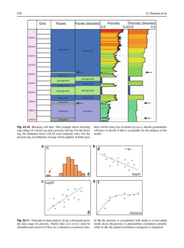
Fig. 22.10 Blocking well data. This example shows blocking
(upscaling) of a facies log and a porosity (ϕ) log. For the facies
log, the dominant facies will be used (majority rule). For the
porosity log, an arithmetic average will be applied. In both cases
there will be some loss of details (arrows), and the geomodeller
will have to decide if that is acceptable for the purpose of the
model
a
b
c
d
Fig. 22.11 Principles in data analysis. In (a), a histogram gives
the data range for porosity. Outlier data (red arrow) must be
identified and removed if they are evaluated as erroneous data.
In (b) the porosity is crossplotted with depth to reveal depth
trends. In (c), the porosity vs. permeability correlation is plotted,
while in (d), the spatial correlation (variogram) is displayed
570
J.C. Rivenæs et al.