

More about Discovery Process Models
63
where x is the pool size, with σ (shape factor) >0, β (spread factor) > 0.
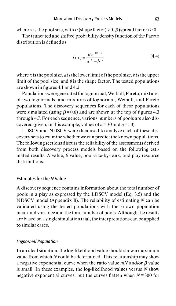
The truncated and shifted probability density function of the Pareto
distribution is defi ned as
− −
−
−
=
−
( 1)
( )
x
f x
a
b
u
u
u
u
(4.4)
where x is the pool size, a is the lower limit of the pool size, b is the upper
limit of the pool size, and θ is the shape factor. The tested populations
are shown in fi gures 4.1 and 4.2.
Populations were generated for lognormal, Weibull, Pareto, mixtures
of two lognormals, and mixtures of lognormal, Weibull, and Pareto
populations. The discovery sequences for each of these populations
were simulated (using β = 0.6) and are shown at the top of fi gures 4.3
through 4.7. For each sequence, various numbers of pools are also discovered (given, in this example, values of n = 30 and n = 50).
LDSCV and NDSCV were then used to analyze each of these discovery sets to examine whether we can predict the known populations.
The following sections discuss the reliability of the assessments derived
from both discovery process models based on the following estimated results: N value, β value, pool-size-by-rank, and play resource
distributions.
Estimates for the N Value
A discovery sequence contains information about the total number of
pools in a play as expressed by the LDSCV model (Eq. 3.5) and the
NDSCV model (Appendix B). The reliability of estimating N can be
validated using the tested populations with the known population
mean and variance and the total number of pools. Although the results
are based on a single simulation trial, the interpretations can be applied
to similar cases.
Lognormal Population
In an ideal situation, the log-likelihood value should show a maximum
value from which N could be determined. This relationship may show
a negative exponential curve when the ratio value n/N and/or β value
is small. In these examples, the log-likelihood values versus N show
negative exponential curves, but the curves fl atten when N = 300 for
63
where x is the pool size, with σ (shape factor) >0, β (spread factor) > 0.
The truncated and shifted probability density function of the Pareto
distribution is defi ned as
− −
−
−
=
−
( 1)
( )
x
f x
a
b
u
u
u
u
(4.4)
where x is the pool size, a is the lower limit of the pool size, b is the upper
limit of the pool size, and θ is the shape factor. The tested populations
are shown in fi gures 4.1 and 4.2.
Populations were generated for lognormal, Weibull, Pareto, mixtures
of two lognormals, and mixtures of lognormal, Weibull, and Pareto
populations. The discovery sequences for each of these populations
were simulated (using β = 0.6) and are shown at the top of fi gures 4.3
through 4.7. For each sequence, various numbers of pools are also discovered (given, in this example, values of n = 30 and n = 50).
LDSCV and NDSCV were then used to analyze each of these discovery sets to examine whether we can predict the known populations.
The following sections discuss the reliability of the assessments derived
from both discovery process models based on the following estimated results: N value, β value, pool-size-by-rank, and play resource
distributions.
Estimates for the N Value
A discovery sequence contains information about the total number of
pools in a play as expressed by the LDSCV model (Eq. 3.5) and the
NDSCV model (Appendix B). The reliability of estimating N can be
validated using the tested populations with the known population
mean and variance and the total number of pools. Although the results
are based on a single simulation trial, the interpretations can be applied
to similar cases.
Lognormal Population
In an ideal situation, the log-likelihood value should show a maximum
value from which N could be determined. This relationship may show
a negative exponential curve when the ratio value n/N and/or β value
is small. In these examples, the log-likelihood values versus N show
negative exponential curves, but the curves fl atten when N = 300 for