

Estimating Mature Plays
59
The play potential distribution (depending on the match, see
Fig. 3.14A) shows that there is a 90% chance with the potential ranging from 3.3 × 10
6 m
3 to 3.5 × 10
6 m
3 , with the mean of the distribution
being 3.4 × 10
6 m
3
. Note that the potential distribution is the sum of all
undiscovered pools from Figure 3.14A, and therefore is very narrow. A
more acceptable range can be derived from the conditional potential,
discussed in the next section.
Probable Play Potential Distribution
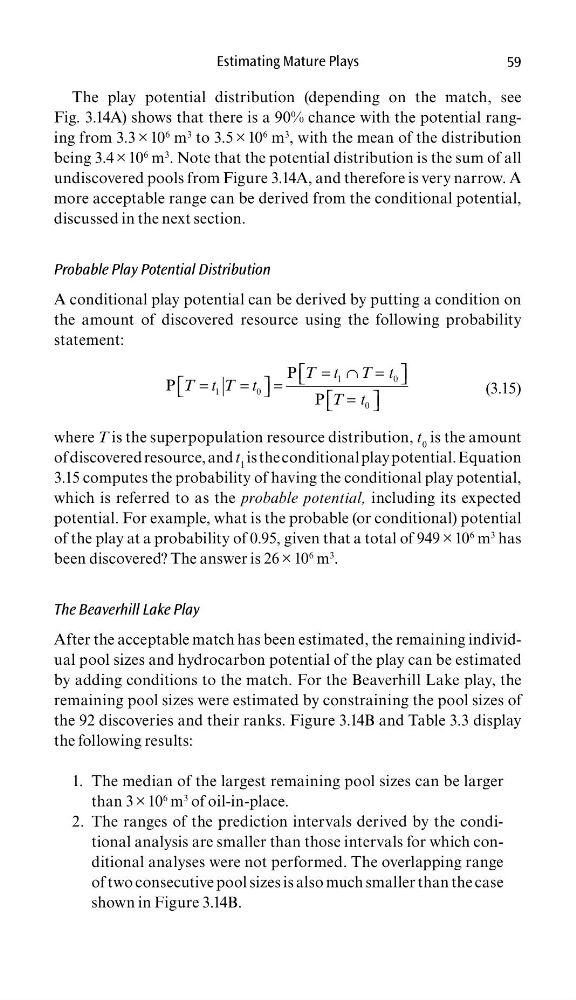
A conditional play potential can be derived by putting a condition on
the amount of discovered resource using the following probability
statement:
1
0
1
0
0
P
P
P
T t T t
T t T t
T t
= ∩ =
=
=
=
=
(3.15)
where T is the superpopulation resource distribution, t 0 is the amount
of discovered resource, and t 1 is the conditional play potential. Equation
3.15 computes the probability of having the conditional play potential,
which is referred to as the probable potential, including its expected
potential. For example, what is the probable (or conditional) potential
of the play at a probability of 0.95, given that a total of 949 × 10
6 m
3 has
been discovered? The answer is 26 × 10
6 m
3
.
The Beaverhill Lake Play
After the acceptable match has been estimated, the remaining individual pool sizes and hydrocarbon potential of the play can be estimated
by adding conditions to the match. For the Beaverhill Lake play, the
remaining pool sizes were estimated by constraining the pool sizes of
the 92 discoveries and their ranks. Figure 3.14B and Table 3.3 display
the following results:
The median of the largest remaining pool sizes can be larger
1.
than 3 × 10
6 m
3 of oil-in-place.
The ranges of the prediction intervals derived by the condi2.
tional analysis are smaller than those intervals for which conditional analyses were not performed. The overlapping range
of two consecutive pool sizes is also much smaller than the case
shown in Figure 3.14B.
59
The play potential distribution (depending on the match, see
Fig. 3.14A) shows that there is a 90% chance with the potential ranging from 3.3 × 10
6 m
3 to 3.5 × 10
6 m
3 , with the mean of the distribution
being 3.4 × 10
6 m
3
. Note that the potential distribution is the sum of all
undiscovered pools from Figure 3.14A, and therefore is very narrow. A
more acceptable range can be derived from the conditional potential,
discussed in the next section.
Probable Play Potential Distribution
A conditional play potential can be derived by putting a condition on
the amount of discovered resource using the following probability
statement:
1
0
1
0
0
P
P
P
T t T t
T t T t
T t
= ∩ =
=
=
=
=
(3.15)
where T is the superpopulation resource distribution, t 0 is the amount
of discovered resource, and t 1 is the conditional play potential. Equation
3.15 computes the probability of having the conditional play potential,
which is referred to as the probable potential, including its expected
potential. For example, what is the probable (or conditional) potential
of the play at a probability of 0.95, given that a total of 949 × 10
6 m
3 has
been discovered? The answer is 26 × 10
6 m
3
.
The Beaverhill Lake Play
After the acceptable match has been estimated, the remaining individual pool sizes and hydrocarbon potential of the play can be estimated
by adding conditions to the match. For the Beaverhill Lake play, the
remaining pool sizes were estimated by constraining the pool sizes of
the 92 discoveries and their ranks. Figure 3.14B and Table 3.3 display
the following results:
The median of the largest remaining pool sizes can be larger
1.
than 3 × 10
6 m
3 of oil-in-place.
The ranges of the prediction intervals derived by the condi2.
tional analysis are smaller than those intervals for which conditional analyses were not performed. The overlapping range
of two consecutive pool sizes is also much smaller than the case
shown in Figure 3.14B.