

Nonparametric Procedure for Estimating Distributions
201
and Nair, 1988). The nonparametric estimator can be obtained by maximizing this likelihood.
Under simple random sampling, the nonparametric estimator of F
is given by the usual edf (empirical distribution function)
:
( )
k
k
n
k z y
n
F y
n
≤
= ∑
(B.2)
This estimator is not valid here, however, because the sampling is
biased. Thus the maximum-likelihood estimator of F for the successive
sampling is now given by
:
ˆ
ˆ
( )
k
n
k
k z y
F y
p
≤
= ∑
(B.3)
where { } 1
K
k k
p = , with
=
=
∑
1
1
K
k
k
p
, maximizes the log likelihood
( )
0
1
1
log
Constant +
log
log
( )
k
N n
K
K
tw z
k
k
k
n
k
k
L
n
p
p e
gtd t
−
∞
−
=
=
=
+
∑
∑
∫
(B.4)
The values 1
ˆ
ˆ
,..., k
p
p are to be determined numerically so that the value
of log L expressed by Equation B.4 is maximized. It can be shown that
the maximized estimate for Equation B.4 is
( )
( )
( )
( )
0
1
( 1)
1
( )
0
1
ˆ
ˆ
( )
ˆ
ˆ
1
ˆ
( )
k
l
l
l
tw z
j
N n
K
tw z
k
l
n
K
tw z
l
l
j
k
l
k
N n
K
tw z
l
n
l
p e
p e
g t dt
p e
n
n
n
p
N N
N
p e
g t dt
−
−
∞
−
−
=
+
=
−
∞
−
=
∑
∑
∑
=
+ −
∫
∫
(B.5)
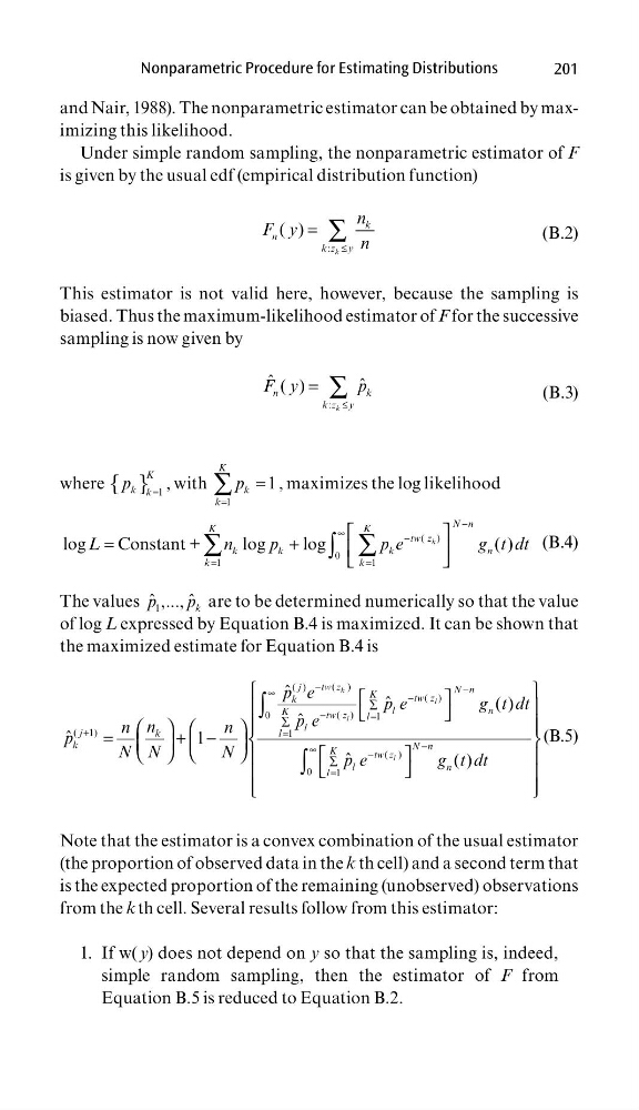
Note that the estimator is a convex combination of the usual estimator
(the proportion of observed data in the k th cell) and a second term that
is the expected proportion of the remaining (unobserved) observations
from the k th cell. Several results follow from this estimator:
If w(
1.
y) does not depend on y so that the sampling is, indeed,
simple random sampling, then the estimator of F from
Equation B.5 is reduced to Equation B.2.
201
and Nair, 1988). The nonparametric estimator can be obtained by maximizing this likelihood.
Under simple random sampling, the nonparametric estimator of F
is given by the usual edf (empirical distribution function)
:
( )
k
k
n
k z y
n
F y
n
≤
= ∑
(B.2)
This estimator is not valid here, however, because the sampling is
biased. Thus the maximum-likelihood estimator of F for the successive
sampling is now given by
:
ˆ
ˆ
( )
k
n
k
k z y
F y
p
≤
= ∑
(B.3)
where { } 1
K
k k
p = , with
=
=
∑
1
1
K
k
k
p
, maximizes the log likelihood
( )
0
1
1
log
Constant +
log
log
( )
k
N n
K
K
tw z
k
k
k
n
k
k
L
n
p
p e
gtd t
−
∞
−
=
=
=
+
∑
∑
∫
(B.4)
The values 1
ˆ
ˆ
,..., k
p
p are to be determined numerically so that the value
of log L expressed by Equation B.4 is maximized. It can be shown that
the maximized estimate for Equation B.4 is
( )
( )
( )
( )
0
1
( 1)
1
( )
0
1
ˆ
ˆ
( )
ˆ
ˆ
1
ˆ
( )
k
l
l
l
tw z
j
N n
K
tw z
k
l
n
K
tw z
l
l
j
k
l
k
N n
K
tw z
l
n
l
p e
p e
g t dt
p e
n
n
n
p
N N
N
p e
g t dt
−
−
∞
−
−
=
+
=
−
∞
−
=
∑
∑
∑
=
+ −
∫
∫
(B.5)
Note that the estimator is a convex combination of the usual estimator
(the proportion of observed data in the k th cell) and a second term that
is the expected proportion of the remaining (unobserved) observations
from the k th cell. Several results follow from this estimator:
If w(
1.
y) does not depend on y so that the sampling is, indeed,
simple random sampling, then the estimator of F from
Equation B.5 is reduced to Equation B.2.