

Estimation of Superpopulation Parameters
195
(
)
( ) (
) (
)
( )
(
)
h l
j l
l
u
l
j
l
u
∞
∞
∞
=
∞
∂
= +
∂
∂
= −
∂
∑
∫
∫
∫
1
0
0
0
0
0
1
P
, ', '
log
, '
, , ', '
1
E
log
, '
, ', '
n
l
r
r
l N n l
f a
a
l
d da
N
n
f A
d
N
d
x
d
␥
␥
␥
(A.67)
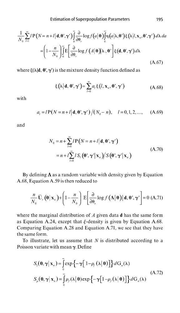
where j(l|d, ', ␥') is the mixture density function defi ned as
(
)
(
)
j l
j
∞
=
= ∑
0
, ', '
, , ', '
l
n
l
a l
d
x
␥
␥
(A.68)
with
0
P
, ', '
,
0,1, 2, ,
(
)(
)
l
a l N n l
N n
l
=
= +
−
=
…
d ␥
(A.69)
and
(
)
(
) (
)
∞
=
∞
=
= +
= +
= +
∑
∑
0
0
0
P
, ' , '
', '
', '
l
l
n
n
l
N n
l N n l
n l lS
S
d
x
x
␥
␥
␥
(A.70)
By defi ning L as a random variable with density given by Equation
A.68, Equation A.59 is then reduced to
( )
( )
0
0
1
E
l o g
, ' , ' 0
r
n
r
n
n
f
N
N
u
∂
+ −
=
∂
U
x
d
⌳
␥
(A.71)
where the marginal distribution of A given data d has the same form
as Equation A.24, except that j-density is given by Equation A.68.
Comparing Equation A.28 and Equation A.71, we see that they have
the same form.
To illustrate, let us assume that N is distributed according to a
Poisson variate with mean ␥. Defi ne
{
}
{
}
1
0
0
,
e x p
1
G( )
,
(
) e x p
1
G( )
(
)
( )
(
)
( )
n
f
n
n
f
f
n
S
d
S
d
l
l
l
l
l
∞
∞
=
−
−
=
−
−
∫
∫
x
x
r
r
r
r
␥
␥
␥
␥
(A.72)
195
(
)
( ) (
) (
)
( )
(
)
h l
j l
l
u
l
j
l
u
∞
∞
∞
=
∞
∂
= +
∂
∂
= −
∂
∑
∫
∫
∫
1
0
0
0
0
0
1
P
, ', '
log
, '
, , ', '
1
E
log
, '
, ', '
n
l
r
r
l N n l
f a
a
l
d da
N
n
f A
d
N
d
x
d
␥
␥
␥
(A.67)
where j(l|d, ', ␥') is the mixture density function defi ned as
(
)
(
)
j l
j
∞
=
= ∑
0
, ', '
, , ', '
l
n
l
a l
d
x
␥
␥
(A.68)
with
0
P
, ', '
,
0,1, 2, ,
(
)(
)
l
a l N n l
N n
l
=
= +
−
=
…
d ␥
(A.69)
and
(
)
(
) (
)
∞
=
∞
=
= +
= +
= +
∑
∑
0
0
0
P
, ' , '
', '
', '
l
l
n
n
l
N n
l N n l
n l lS
S
d
x
x
␥
␥
␥
(A.70)
By defi ning L as a random variable with density given by Equation
A.68, Equation A.59 is then reduced to
( )
( )
0
0
1
E
l o g
, ' , ' 0
r
n
r
n
n
f
N
N
u
∂
+ −
=
∂
U
x
d
⌳
␥
(A.71)
where the marginal distribution of A given data d has the same form
as Equation A.24, except that j-density is given by Equation A.68.
Comparing Equation A.28 and Equation A.71, we see that they have
the same form.
To illustrate, let us assume that N is distributed according to a
Poisson variate with mean ␥. Defi ne
{
}
{
}
1
0
0
,
e x p
1
G( )
,
(
) e x p
1
G( )
(
)
( )
(
)
( )
n
f
n
n
f
f
n
S
d
S
d
l
l
l
l
l
∞
∞
=
−
−
=
−
−
∫
∫
x
x
r
r
r
r
␥
␥
␥
␥
(A.72)