

Estimation of Superpopulation Parameters
179
which is simply the likelihood of the infi nite population selection-biased
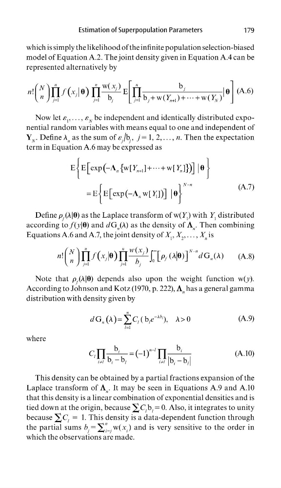
model of Equation A.2. The joint density given in Equation A.4 can be
represented alternatively by
( )
=
=
=
+
+
+ +
∏
∏
∏
"
1
1
1
1
w( )
b
!
E
b
b w(
)
w( )
n
n
n
j
j
j
j
j
j
j
j
n
N
N
n
x
n
f x
Y
Y
(A.6)
Now let « 1 , . . . , « N be independent and identically distributed exponential random variables with means equal to one and independent of
Y N . Defi ne l n as the sum of « j / b j , j 5 1, 2, . . . , n. Then the expectation
term in Equation A.6 may be expressed as
{
}
(
)
(
)
+
−
−
+ +
=
−
"
1
1
E E exp
w[
]
w[ ]
E E exp
w[ ]
n
n
n
N n
n
Y
Y
Y
⌳
⌳
(A.7)
Defi ne r f (l|) as the Laplace transform of w(Y 1 ) with Y 1 distributed
according to f (y|) and d G n (l) as the density of L n . Then combining
Equations A.6 and A.7, the joint density of X 1 , X 2 , . . . , X n is
( )
∞
−
=
=
∏
∏
∫ 0
1
1
( )
!
()
G ( )
n
n
N n
j
j
f
n
j
j
j
N
n
w x
n
f x
d
b
r l
l
(A.8)
Note that r f (l|) depends also upon the weight function w(y).
According to Johnson and Kotz (1970, p. 222), L n has a general gamma
distribution with density given by
( )
−
=
=
>
∑
1
G
(b
) ,
0
l
n
b
n
l
l
l
d
C
e
l
l
l
(A.9)
where
( )
−
≠
≠
= −
−
−
∏
∏
b
b
1
b b
b b
n l
i
i
l
i l
i l
i
l
i
l
C
(A.10)
This density can be obtained by a partial fractions expansion of the
Laplace transform of L n . It may be seen in Equations A.9 and A.10
that this density is a linear combination of exponential densities and is
tied down at the origin, because S C l b l 5 0. Also, it integrates to unity
because S C l 5 1. This density is a data-dependent function through
the partial sums b j 5 S
n
i5j
w( x i ) and is very sensitive to the order in
which the observations are made.
179
which is simply the likelihood of the infi nite population selection-biased
model of Equation A.2. The joint density given in Equation A.4 can be
represented alternatively by
( )
=
=
=
+
+
+ +
∏
∏
∏
"
1
1
1
1
w( )
b
!
E
b
b w(
)
w( )
n
n
n
j
j
j
j
j
j
j
j
n
N
N
n
x
n
f x
Y
Y
(A.6)
Now let « 1 , . . . , « N be independent and identically distributed exponential random variables with means equal to one and independent of
Y N . Defi ne l n as the sum of « j / b j , j 5 1, 2, . . . , n. Then the expectation
term in Equation A.6 may be expressed as
{
}
(
)
(
)
+
−
−
+ +
=
−
"
1
1
E E exp
w[
]
w[ ]
E E exp
w[ ]
n
n
n
N n
n
Y
Y
Y
⌳
⌳
(A.7)
Defi ne r f (l|) as the Laplace transform of w(Y 1 ) with Y 1 distributed
according to f (y|) and d G n (l) as the density of L n . Then combining
Equations A.6 and A.7, the joint density of X 1 , X 2 , . . . , X n is
( )
∞
−
=
=
∏
∏
∫ 0
1
1
( )
!
()
G ( )
n
n
N n
j
j
f
n
j
j
j
N
n
w x
n
f x
d
b
r l
l
(A.8)
Note that r f (l|) depends also upon the weight function w(y).
According to Johnson and Kotz (1970, p. 222), L n has a general gamma
distribution with density given by
( )
−
=
=
>
∑
1
G
(b
) ,
0
l
n
b
n
l
l
l
d
C
e
l
l
l
(A.9)
where
( )
−
≠
≠
= −
−
−
∏
∏
b
b
1
b b
b b
n l
i
i
l
i l
i l
i
l
i
l
C
(A.10)
This density can be obtained by a partial fractions expansion of the
Laplace transform of L n . It may be seen in Equations A.9 and A.10
that this density is a linear combination of exponential densities and is
tied down at the origin, because S C l b l 5 0. Also, it integrates to unity
because S C l 5 1. This density is a data-dependent function through
the partial sums b j 5 S
n
i5j
w( x i ) and is very sensitive to the order in
which the observations are made.