

120
Statistical Methods for Estimating Petroleum Resources
=
∑
ln(Constant) +
i
i
m
m
(5.11)
<
=
+
∑
∑∑
2
2
2
i
i j
i j
s
s
s
(5.12)
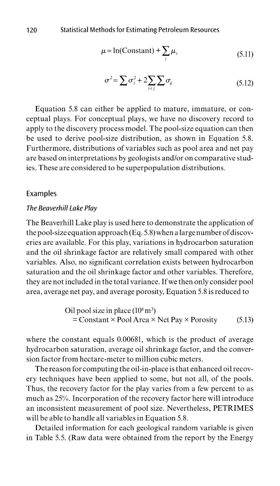
Equation 5.8 can either be applied to mature, immature, or conceptual plays. For conceptual plays, we have no discovery record to
apply to the discovery process model. The pool-size equation can then
be used to derive pool-size distribution, as shown in Equation 5.8.
Furthermore, distributions of variables such as pool area and net pay
are based on interpretations by geologists and/or on comparative studies. These are considered to be superpopulation distributions.
Examples
The Beaverhill Lake Play
The Beaverhill Lake play is used here to demonstrate the application of
the pool-size equation approach (Eq. 5.8) when a large number of discoveries are available. For this play, variations in hydrocarbon saturation
and the oil shrinkage factor are relatively small compared with other
variables. Also, no signifi cant correlation exists between hydrocarbon
saturation and the oil shrinkage factor and other variables. Therefore,
they are not included in the total variance. If we then only consider pool
area, average net pay, and average porosity, Equation 5.8 is reduced to
Oil pool size in place (10
6 m
3
)
= Constant × Pool Area × Net Pay × Porosity
(5.13)
where the constant equals 0.00681, which is the product of average
hydrocarbon saturation, average oil shrinkage factor, and the conversion factor from hectare-meter to million cubic meters.
The reason for computing the oil-in-place is that enhanced oil recovery techniques have been applied to some, but not all, of the pools.
Thus, the recovery factor for the play varies from a few percent to as
much as 25%. Incorporation of the recovery factor here will introduce
an inconsistent measurement of pool size. Nevertheless, PETRIMES
will be able to handle all variables in Equation 5.8.
Detailed information for each geological random variable is given
in Table 5.5. (Raw data were obtained from the report by the Energy
Statistical Methods for Estimating Petroleum Resources
=
∑
ln(Constant) +
i
i
m
m
(5.11)
<
=
+
∑
∑∑
2
2
2
i
i j
i j
s
s
s
(5.12)
Equation 5.8 can either be applied to mature, immature, or conceptual plays. For conceptual plays, we have no discovery record to
apply to the discovery process model. The pool-size equation can then
be used to derive pool-size distribution, as shown in Equation 5.8.
Furthermore, distributions of variables such as pool area and net pay
are based on interpretations by geologists and/or on comparative studies. These are considered to be superpopulation distributions.
Examples
The Beaverhill Lake Play
The Beaverhill Lake play is used here to demonstrate the application of
the pool-size equation approach (Eq. 5.8) when a large number of discoveries are available. For this play, variations in hydrocarbon saturation
and the oil shrinkage factor are relatively small compared with other
variables. Also, no signifi cant correlation exists between hydrocarbon
saturation and the oil shrinkage factor and other variables. Therefore,
they are not included in the total variance. If we then only consider pool
area, average net pay, and average porosity, Equation 5.8 is reduced to
Oil pool size in place (10
6 m
3
)
= Constant × Pool Area × Net Pay × Porosity
(5.13)
where the constant equals 0.00681, which is the product of average
hydrocarbon saturation, average oil shrinkage factor, and the conversion factor from hectare-meter to million cubic meters.
The reason for computing the oil-in-place is that enhanced oil recovery techniques have been applied to some, but not all, of the pools.
Thus, the recovery factor for the play varies from a few percent to as
much as 25%. Incorporation of the recovery factor here will introduce
an inconsistent measurement of pool size. Nevertheless, PETRIMES
will be able to handle all variables in Equation 5.8.
Detailed information for each geological random variable is given
in Table 5.5. (Raw data were obtained from the report by the Energy