

94
Statistical Methods for Estimating Petroleum Resources
have also been tested using Q–Q plots. Some of the outliers contained
in the samples might not follow straight lines. However if the outliers
are excluded from the Q–Q plots, one can make the following conclusions from observations of more than 100 plays:
In all cases, lognormal distributions are the most appropri1.
ate distributions for the plays tested, as shown in fi gures 4.22
and 4.23.
Generally, the Weibull distribution exhibits a concave curve
2.
in the Q–Q plots. Figure 4.24 shows that it is the best distribution for this play. This is one of only two plays from more
than 100 plays studied for which the Weibull distribution is
best. However, the lognormal or power normal distributions
are also appropriate.
In the Pareto Q–Q plots, all the play data sets are compressed
3.
into a small area in the lower left end of the plot. An exception
is that presented in Figure 4.25, which shows that the Pareto
distribution is the best of the four for this play. This is the only
play from more than 100 plays studied for which the Pareto
distribution is best. The Pareto distribution may sometimes be
adequate for the largest few pools (Fig. 4.26).
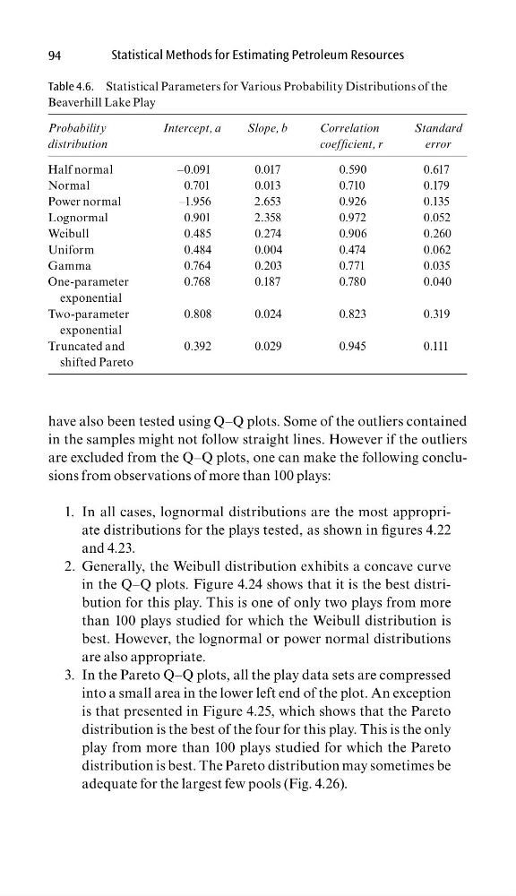
Table 4.6. Statistical Parameters for Various Probability Distributions of the
Beaverhill Lake Play
Probability
distribution
Intercept, a
Slope, b
Correlation
coeffi cient, r
Standard
error
Half normal
–0.091
0.017
0.590
0.617
Normal
0.701
0.013
0.710
0.179
Power normal
–1.956
2.653
0.926
0.135
Lognormal
0.901
2.358
0.972
0.052
Weibull
0.485
0.274
0.906
0.260
Uniform
0.484
0.004
0.474
0.062
Gamma
0.764
0.203
0.771
0.035
One-parameter
exponential
0.768
0.187
0.780
0.040
Two-parameter
exponential
0.808
0.024
0.823
0.319
Truncated and
shifted Pareto
0.392
0.029
0.945
0.111
Statistical Methods for Estimating Petroleum Resources
have also been tested using Q–Q plots. Some of the outliers contained
in the samples might not follow straight lines. However if the outliers
are excluded from the Q–Q plots, one can make the following conclusions from observations of more than 100 plays:
In all cases, lognormal distributions are the most appropri1.
ate distributions for the plays tested, as shown in fi gures 4.22
and 4.23.
Generally, the Weibull distribution exhibits a concave curve
2.
in the Q–Q plots. Figure 4.24 shows that it is the best distribution for this play. This is one of only two plays from more
than 100 plays studied for which the Weibull distribution is
best. However, the lognormal or power normal distributions
are also appropriate.
In the Pareto Q–Q plots, all the play data sets are compressed
3.
into a small area in the lower left end of the plot. An exception
is that presented in Figure 4.25, which shows that the Pareto
distribution is the best of the four for this play. This is the only
play from more than 100 plays studied for which the Pareto
distribution is best. The Pareto distribution may sometimes be
adequate for the largest few pools (Fig. 4.26).
Table 4.6. Statistical Parameters for Various Probability Distributions of the
Beaverhill Lake Play
Probability
distribution
Intercept, a
Slope, b
Correlation
coeffi cient, r
Standard
error
Half normal
–0.091
0.017
0.590
0.617
Normal
0.701
0.013
0.710
0.179
Power normal
–1.956
2.653
0.926
0.135
Lognormal
0.901
2.358
0.972
0.052
Weibull
0.485
0.274
0.906
0.260
Uniform
0.484
0.004
0.474
0.062
Gamma
0.764
0.203
0.771
0.035
One-parameter
exponential
0.768
0.187
0.780
0.040
Two-parameter
exponential
0.808
0.024
0.823
0.319
Truncated and
shifted Pareto
0.392
0.029
0.945
0.111