

5.6 Prototypical Implementation
141
stop the simulation. The observation period is set to one month in the experiment
properties (Figure 5.36).
AnyLogic offers the option to define constraints and restrictions for the optimization experiment. While constraints are tested before the simulation run is
started, restrictions are tested afterwards and depending on the outcome of a test
the simulation run is counted as feasible or non-feasible solution. The restrictions are important for the test case, since it has to be avoided that any energy
savings are achieved at the expense of a lower output quantity. Thus, only parameter variations for an output quantity of 2.100 pieces 10 or higher are counted as
feasible solutions.
Since the defined parameters all have a comparatively large variance range, it
makes sense to run through a high number of iterations in order to determine an
ideal parameter set for the given objective. As the number of iterations in AnyLogic’s PLE is limited to 500, this maximum allowed number is used. The setup
of replications is not required in this scenario because the model does not contain
any stochastic elements. When all parameters and setups have been defined the
optimization experiment can be started to depict the ideal switching times for the
defined parameters. The optimization experiment contains a graphical analysis
of the tested parameter variants, showing feasible, infeasible and current parameter sets. After the completion of all iterations, the best parameter set can be
directly copied into the simulation model setup to run the simulation model with
the optimal parameter setting (Figure 5.37).
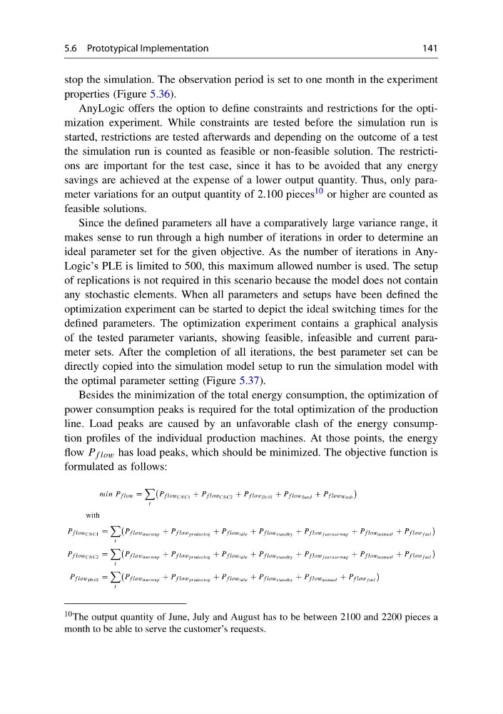
Besides the minimization of the total energy consumption, the optimization of
power consumption peaks is required for the total optimization of the production
line. Load peaks are caused by an unfavorable clash of the energy consumption profiles of the individual production machines. At those points, the energy
flow P f low has load peaks, which should be minimized. The objective function is
formulated as follows:
min Pf low =
t
Pf lowCNC1 + Pf lowCNC2 + Pf lowDrill + Pf lowSand + Pf lowWash
with
Pf lowCNC1 =
t
Pf lowwarmup + Pf lowproducing + Pf lowidle + Pf lowstandby + Pf low f astwarmup + Pf lowmanual + Pf low f ail
Pf lowCNC2 =
t
Pf lowwarmup + Pf lowproducing + Pf lowidle + Pf lowstandby + Pf low f astwarmup + Pf lowmanual + Pf low f ail
Pf lowDrill =
t
Pf lowwarmup + Pf lowproducing + Pf lowidle + Pf lowstandby + Pf lowmanual + Pf low f ail
10 The output quantity of June, July and August has to be between 2100 and 2200 pieces a
month to be able to serve the customer’s requests.
141
stop the simulation. The observation period is set to one month in the experiment
properties (Figure 5.36).
AnyLogic offers the option to define constraints and restrictions for the optimization experiment. While constraints are tested before the simulation run is
started, restrictions are tested afterwards and depending on the outcome of a test
the simulation run is counted as feasible or non-feasible solution. The restrictions are important for the test case, since it has to be avoided that any energy
savings are achieved at the expense of a lower output quantity. Thus, only parameter variations for an output quantity of 2.100 pieces 10 or higher are counted as
feasible solutions.
Since the defined parameters all have a comparatively large variance range, it
makes sense to run through a high number of iterations in order to determine an
ideal parameter set for the given objective. As the number of iterations in AnyLogic’s PLE is limited to 500, this maximum allowed number is used. The setup
of replications is not required in this scenario because the model does not contain
any stochastic elements. When all parameters and setups have been defined the
optimization experiment can be started to depict the ideal switching times for the
defined parameters. The optimization experiment contains a graphical analysis
of the tested parameter variants, showing feasible, infeasible and current parameter sets. After the completion of all iterations, the best parameter set can be
directly copied into the simulation model setup to run the simulation model with
the optimal parameter setting (Figure 5.37).
Besides the minimization of the total energy consumption, the optimization of
power consumption peaks is required for the total optimization of the production
line. Load peaks are caused by an unfavorable clash of the energy consumption profiles of the individual production machines. At those points, the energy
flow P f low has load peaks, which should be minimized. The objective function is
formulated as follows:
min Pf low =
t
Pf lowCNC1 + Pf lowCNC2 + Pf lowDrill + Pf lowSand + Pf lowWash
with
Pf lowCNC1 =
t
Pf lowwarmup + Pf lowproducing + Pf lowidle + Pf lowstandby + Pf low f astwarmup + Pf lowmanual + Pf low f ail
Pf lowCNC2 =
t
Pf lowwarmup + Pf lowproducing + Pf lowidle + Pf lowstandby + Pf low f astwarmup + Pf lowmanual + Pf low f ail
Pf lowDrill =
t
Pf lowwarmup + Pf lowproducing + Pf lowidle + Pf lowstandby + Pf lowmanual + Pf low f ail
10 The output quantity of June, July and August has to be between 2100 and 2200 pieces a
month to be able to serve the customer’s requests.